
🤵♂️ 个人主页:@艾派森的个人主页
✍🏻作者简介:Python学习者
🐋 希望大家多多支持,我们一起进步!😄
如果文章对你有帮助的话,
欢迎评论 💬点赞👍🏻 收藏 📂加关注+
目录
1.项目背景
2.数据获取
3.技术工具
4.实验过程
4.1导入数据
4.2数据预处理
4.3数据可视化
4.4特征工程
4.5构建模型
4.6特征重要性
4.7模型预测
源代码
1.项目背景
随着互联网技术的快速发展,网络已经成为人们获取信息、交流互动的重要平台。在房地产领域,尤其是在租房市场中,大量的租房信息涌现在各大租房网站和平台上。然而,这些海量的数据往往分散、不规范,难以直接用于分析和预测。因此,如何有效地从这些数据中提取有价值的信息,进而对租房价格进行预测和优化,成为了一个亟待解决的问题。
杭州作为中国的经济发达城市,人口流动性大,租房市场活跃。然而,租房价格的波动往往受到多种因素的影响,如房屋的位置、面积、装修情况、配套设施等。这些因素之间相互作用,使得租房价格的预测变得复杂而困难。传统的预测方法往往基于经验或者简单的统计分析,难以准确捕捉价格变动的规律。
Python作为一种强大的编程语言,具有简洁易读、功能强大等特点,在数据处理、爬虫、机器学习等领域有着广泛的应用。通过Python爬虫技术,我们可以从租房网站上抓取大量的租房信息,包括房屋的描述、价格、位置等。而机器学习技术则可以从这些数据中学习出价格变动的规律,进而构建出预测模型。
因此,本研究旨在结合Python爬虫和机器学习技术,对杭州租房价格进行预测建模与优化研究。通过抓取租房网站上的数据,提取出影响租房价格的关键因素,并利用机器学习算法构建预测模型。通过对模型的优化和验证,我们可以更加准确地预测租房价格,为租房者和房东提供有价值的参考信息,同时也为房地产市场的研究和决策提供数据支持。
2.数据获取
本次实验的数据集来源于房天下中杭州的租房数据
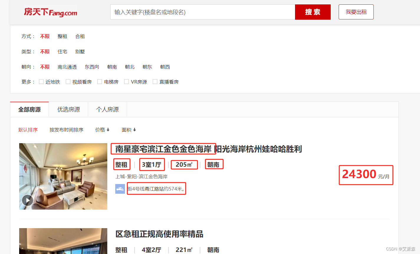
通过分析网页的结构,我们发现列表页中的数据并不满足需求,所以我们需要进入详情页,然后使用xpath进行数据提取。故我们写爬虫代码的思路就是先用requests库发送列表页请求,使用xpath获取列表页中各详情页的url,然后再次发送详情页请求,使用xpath提取返回内容中的数据,最后再加个多页爬取并将数据保存再本地即可。
定义爬虫主函数,获取详情页url
def main(page,f):
    url = f'https://{city_en}.zu.fang.com/house/i3{page}/?rfss=1-9988c4a227ce113113-a6'
    resp = requests.get(url,headers=headers)
    tree = etree.HTML(resp.text)
    dl_list = tree.xpath('//div[@]/dl')
    print(len(dl_list))
    if len(dl_list) == 0:
        print('IP异常!验证码警告!请返回官网刷新验证码!')
        raise
    else:
        for dl in dl_list:
            href = dl.xpath('./dt/a/@href')[0]
            href = f'https://{city_en}.zu.fang.com' + href
            try:
                get_details(href)
                f.flush()
                time.sleep(random.random())
            except Exception as e:
                print(e)
                pass
定义一个获取详情页的函数
def get_details(url):
    headers['referer'] = 'referer: http://search.fang.com/'
    resp = requests.get(url,headers=headers)
    tree = etree.HTML(resp.text)
    # 城市
    city_ = city
    # 房屋租金
    try:
        house_price = tree.xpath('/html/body/div[5]/div[1]/div[5]/div[1]/div/i/text()')[0] + '元/月'
    except:
        house_price = '暂无数据'
    # 交付方式
    try:
        pay_type = tree.xpath('/html/body/div[5]/div[1]/div[5]/div[1]/div/a/text()')[0]
    except:
        pay_type = '暂无数据'
    # 出租方式
    try:
        hire_style = tree.xpath('/html/body/div[5]/div[1]/div[5]/div[2]/div[1]/div[1]/a/text()')[0]
    except:
        hire_style = '暂无数据'
    # 房屋户型
    try:
        house_type = tree.xpath('/html/body/div[5]/div[1]/div[5]/div[2]/div[2]/div[1]/text()')[0]
    except:
        house_type = '暂无数据'
    # 房屋面积
    try:
        house_area = tree.xpath('/html/body/div[5]/div[1]/div[5]/div[2]/div[3]/div[1]/text()')[0]
    except:
        house_area = '暂无数据'
    # 房屋朝向
    try:
        house_direct = tree.xpath('/html/body/div[5]/div[1]/div[5]/div[3]/div[1]/div[1]/text()')[0]
    except:
        house_direct = '暂无数据'
    # 楼层
    try:
        floor = tree.xpath('/html/body/div[5]/div[1]/div[5]/div[3]/div[2]/div[1]/a/text()')[0]
    except:
        floor = '暂无数据'
    # 房屋装修
    try:
        house_dec = tree.xpath('/html/body/div[5]/div[1]/div[5]/div[3]/div[3]/div[1]/a/text()')[0]
    except:
        house_dec = '暂无数据'
    # 小区
    try:
        xiaoqu = tree.xpath('//*[@id="agantzfxq_C02_07"]/text()')[0]
    except:
        xiaoqu = '暂无数据'
    # 距地铁距离
    try:
        subway_meter = tree.xpath('/html/body/div[5]/div[1]/div[5]/div[4]/div[2]/div/a/text()')[0]
    except:
        subway_meter = '暂无数据'
    # 地址
    try:
        place = tree.xpath('/html/body/div[5]/div[1]/div[5]/div[4]/div[3]/div[2]/a/text()')[0]
    except:
        place = '暂无数据'
    # 配套设施
    try:
        other_fac_list = tree.xpath('/html/body/div[5]/div[2]/div[1]/div[2]/div[2]/ul/li/text()')
        other_fac = ' '.join(other_fac_list)
    except:
        other_fac = '暂无数据 '
    # 房源亮点
    try:
        house_light = tree.xpath('/html/body/div[5]/div[2]/div[1]/div[1]/div[2]/div/div/ul/li[1]/div[2]/text()')[0]
    except:
        house_light = '暂无数据'
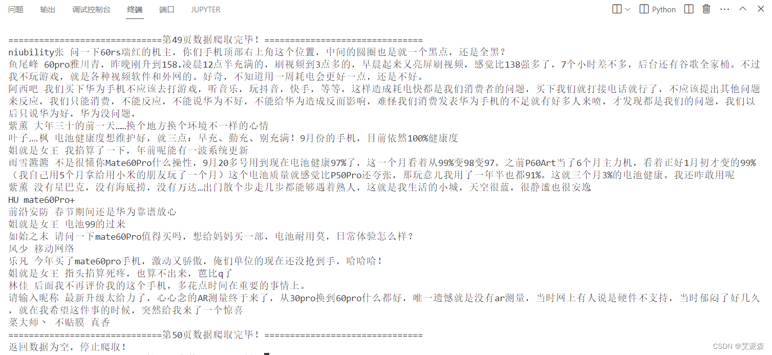
代码运行结果如下:
最后保存的数据文件如下:
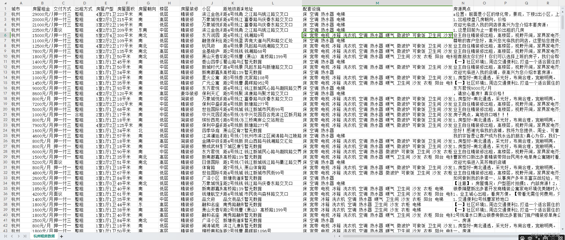
注:完整爬取代码请关注文末公主号后加入QQ粉丝群领取!
3.技术工具
Python版本:3.9
代码编辑器:jupyter notebook
4.实验过程
4.1导入数据
首先导入本次实验用到的第三方库并加载数据集
import matplotlib.pylab as plt
import numpy as np
import seaborn as sns
import pandas as pd
plt.rcParams['font.sans-serif'] = ['SimHei'] #解决中文显示
plt.rcParams['axes.unicode_minus'] = False #解决符号无法显示
sns.set(font='SimHei')
import warnings
warnings.filterwarnings('ignore')
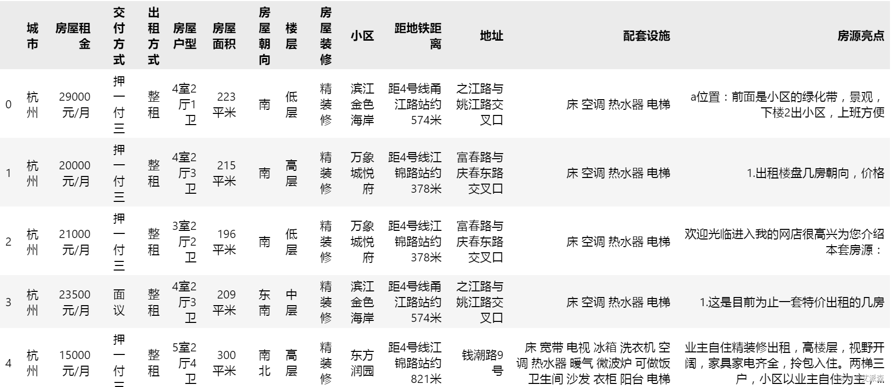
df = pd.read_csv('杭州租房数据.csv')
df.head()
查看数据大小
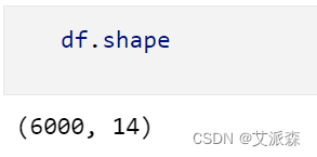
可以看出数据是共有6000条,14个变量

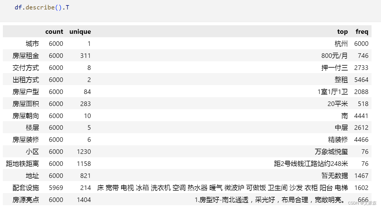
查看数据描述性统计
4.2数据预处理
统计缺失值情况

可以发现配套设施变量中有31个缺失值
统计重复值情况
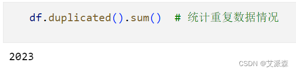
可以发现数据集中共有2023条重复数据。
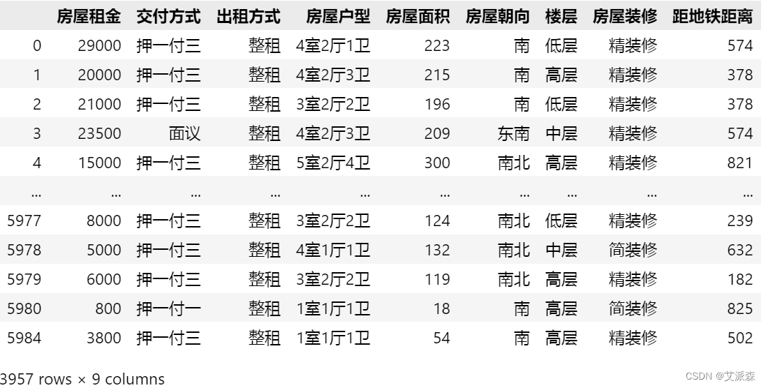
删除缺失值和重复值
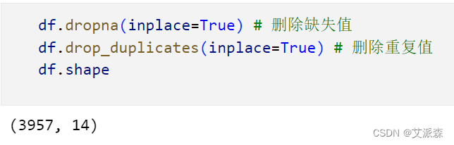
经过清洗之后还剩3957条有效数据。
处理租金数据的格式
df['房屋租金'] = df['房屋租金'].apply(lambda x:int(x.split('元')[0]))
df['房屋租金']

处理房屋面积的格式
df['房屋面积'] = df['房屋面积'].apply(lambda x:int(x[:-2]))
df['房屋面积']
处理距离地铁距离,提取出数字
def subway_distance(x):
    try:
        result = x.split('约')[1].split('米')[0]
    except:
        result = 0
    return int(result)
df['距地铁距离'] = df['距地铁距离'].apply(subway_distance)
df['距地铁距离']
4.3数据可视化
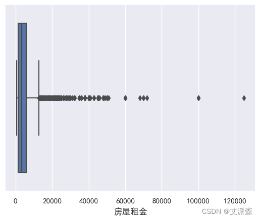
sns.boxplot(data=df,x='房屋租金')
plt.show()
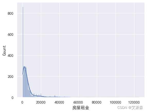
sns.histplot(data=df,x='房屋租金',kde=True)
plt.show()
sns.histplot(data=df,x='房屋面积',kde=True)
plt.show()

plt.scatter(x=df['房屋面积'],y=df['房屋租金'])
plt.show()

sns.countplot(data=df,x='交付方式')
plt.show()

df['出租方式'].value_counts().plot(kind='pie',autopct='%.2f%%')
plt.show()

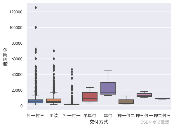
sns.boxplot(data=df,y='房屋租金',x='交付方式')
plt.show()
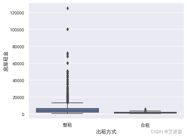
sns.boxplot(data=df,y='房屋租金',x='出租方式')
plt.show()
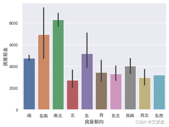
sns.barplot(data=df,x='房屋朝向',y='房屋租金')
plt.show()
df['楼层'].value_counts().plot(kind='pie',autopct='%.2f%%')
plt.show()

sns.barplot(data=df,x='楼层',y='房屋租金')
plt.show()

# 相关性分析
sns.heatmap(df.corr(),vmax=1,annot=True,linewidths=0.5,cbar=False,cmap='YlGnBu',annot_kws={'fontsize':18})
plt.xticks(fontsize=20)
plt.yticks(fontsize=20)
plt.title('各个因素之间的相关系数',fontsize=20)
plt.show()

绘制房源亮点词云图
import jieba
import collections
import re
import stylecloud
from PIL import Image
def draw_WorldCloud(df,pic_name,color='black'):
    data =  ''.join([item for item in df])
    # 文本预处理 :去除一些无用的字符只提取出中文出来
    new_data = re.findall('[\u4e00-\u9fa5]+', data, re.S)
    new_data = "".join(new_data)
    # 文本分词
    seg_list_exact = jieba.cut(new_data, cut_all=True)
    result_list = []
    with open('停用词库.txt', encoding='utf-8') as f: #可根据需要打开停用词库,然后加上不想显示的词语
        con = f.readlines()
        stop_words = set()
        for i in con:
            i = i.replace("\n", "")   # 去掉读取每一行数据的\n
            stop_words.add(i)
    for word in seg_list_exact:
        if word not in stop_words and len(word) > 1:
            result_list.append(word)
    word_counts = collections.Counter(result_list)
    # 词频统计:获取前100最高频的词
    word_counts_top = word_counts.most_common(100)
    print(word_counts_top)
    # 绘制词云图
    stylecloud.gen_stylecloud(text=' '.join(result_list[:500]), # 提取500个词进行绘图
                            collocations=False, # 是否包括两个单词的搭配(二字组)
                            font_path=r'C:\Windows\Fonts\msyh.ttc', #设置字体,参考位置为  C:\Windows\Fonts\ ,根据里面的字体编号来设置
                            size=800, # stylecloud 的大小
                            palette='cartocolors.qualitative.Bold_7', # 调色板,调色网址: https://jiffyclub.github.io/palettable/
                            background_color=color, # 背景颜色
                            icon_name='fas fa-circle', # 形状的图标名称 蒙版网址:https://fontawesome.com/icons?d=gallery&p=2&c=chat,shopping,travel&m=free
                            gradient='horizontal', # 梯度方向
                            max_words=2000, # stylecloud 可包含的最大单词数
                            max_font_size=150, # stylecloud 中的最大字号
                            stopwords=True, # 布尔值,用于筛除常见禁用词
                            output_name=f'{pic_name}.png') # 输出图片
    # 打开图片展示
    img=Image.open(f'{pic_name}.png')
    img.show()
draw_WorldCloud(df['房源亮点'],'房源亮点词云图') # 词云图可视化

4.4特征工程
筛选特征
# 特征筛选
new_df = df[['房屋租金', '交付方式', '出租方式', '房屋户型', '房屋面积', '房屋朝向', '楼层', '房屋装修','距地铁距离']]
new_df
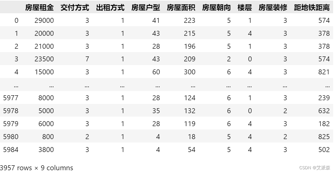
编码处理
# 编码处理
from sklearn.preprocessing import LabelEncoder
for col in new_df.describe(include='O').columns.to_list():
    new_df[col] = LabelEncoder().fit_transform(new_df[col])
new_df
准备建模数据,并拆分数据集为训练集和测试集
from sklearn.model_selection import train_test_split
# 准备数据
X = new_df.drop('房屋租金',axis=1)
y = new_df['房屋租金']
# 划分数据集
X_train,X_test,y_train,y_test = train_test_split(X,y,test_size=0.2,random_state=42)
print('训练集大小:',X_train.shape[0])
print('测试集大小:',X_test.shape[0])

4.5构建模型
先定义一个训练并输出模型指标的函数
from sklearn.metrics import r2_score,mean_absolute_error,mean_squared_error
# 定义一个训练模型并输出模型的评估指标
def train_model(ml_model):
    print("Model is: ", ml_model)
    model = ml_model.fit(X_train, y_train)
    print("Training score: ", model.score(X_train,y_train))
    predictions = model.predict(X_test)
    r2score = r2_score(y_test, predictions)
    print("r2 score is: ", r2score)
    print('MAE:', mean_absolute_error(y_test,predictions))
    print('MSE:', mean_squared_error(y_test,predictions))
    print('RMSE:', np.sqrt(mean_squared_error(y_test,predictions)))
    # 真实值和预测值的差值
    sns.distplot(y_test - predictions)
构建多元回归模型
# 构建多元线性回归
from sklearn.linear_model import LinearRegression
lg = LinearRegression()
train_model(lg)


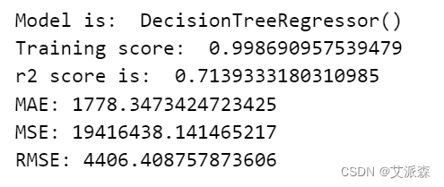
构建决策树回归模型
# 构建决策树回归
from sklearn.tree import DecisionTreeRegressor
tree = DecisionTreeRegressor()
train_model(tree)

构建XGBoost回归模型
# 构建xgboost回归模型
from xgboost import XGBRegressor
xgb = XGBRegressor()
train_model(xgb)
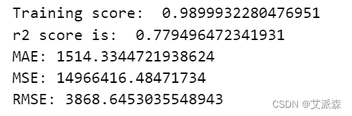

通过对比三个模型的指标,我们发现xgboost模型拟合效果最好,故我们最终选择其作为最终模型。
4.6特征重要性
# 特征重要性评分
feat_labels = X_train.columns[0:]
importances = xgb.feature_importances_
indices = np.argsort(importances)[::-1]
index_list = []
value_list = []
for f,j in zip(range(X_train.shape[1]),indices):
    index_list.append(feat_labels[j])
    value_list.append(importances[j])
    print(f + 1, feat_labels[j], importances[j])
plt.figure(figsize=(10,6))
plt.barh(index_list[::-1],value_list[::-1])
plt.yticks(fontsize=12)
plt.title('各特征重要程度排序',fontsize=14)
plt.show()


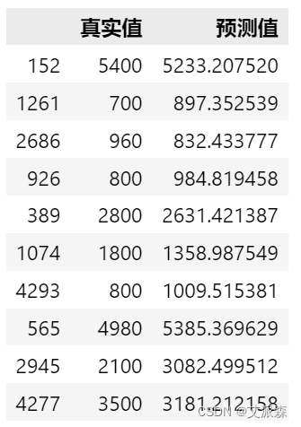
4.7模型预测
# 模型预测
y_pred = xgb.predict(X_test)
result_df = pd.DataFrame()
result_df['真实值'] = y_test
result_df['预测值'] = y_pred
result_df.head(10)
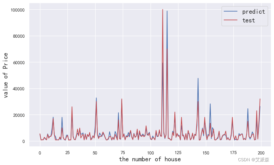
预测结果可视化
# 模型预测可视化
plt.figure(figsize=(10,6))
plt.plot(range(len(y_test))[:200],y_pred[:200],'b',label='predict')
plt.plot(range(len(y_test))[:200],y_test[:200],'r',label='test')
plt.legend(loc='upper right',fontsize=15)
plt.xlabel('the number of house',fontdict={'weight': 'normal', 'size': 15})
plt.ylabel('value of Price',fontdict={'weight': 'normal', 'size': 15})
plt.show()
源代码
import matplotlib.pylab as plt
import numpy as np
import seaborn as sns
import pandas as pd
plt.rcParams['font.sans-serif'] = ['SimHei'] #解决中文显示
plt.rcParams['axes.unicode_minus'] = False   #解决符号无法显示
sns.set(font='SimHei')
import warnings
warnings.filterwarnings('ignore')
df = pd.read_csv('杭州租房数据.csv')
df.head()
df.shape
df.info()
df.describe().T
df.isnull().sum() # 统计缺失值情况
df.duplicated().sum()  # 统计重复数据情况
df.dropna(inplace=True) # 删除缺失值
df.drop_duplicates(inplace=True) # 删除重复值
df.shape
df['房屋租金'] = df['房屋租金'].apply(lambda x:int(x.split('元')[0]))
df['房屋租金']
df['房屋面积'] = df['房屋面积'].apply(lambda x:int(x[:-2]))
df['房屋面积']
sns.boxplot(data=df,x='房屋租金')
plt.show()
sns.histplot(data=df,x='房屋租金',kde=True)
plt.show()
sns.boxplot(data=df,y='房屋面积')
plt.show()
sns.histplot(data=df,x='房屋面积',kde=True)
plt.show()
plt.scatter(x=df['房屋面积'],y=df['房屋租金'])
plt.show()
df['交付方式'].value_counts()
sns.countplot(data=df,x='交付方式')
plt.show()
df['出租方式'].value_counts().plot(kind='pie',autopct='%.2f%%')
plt.show()
sns.boxplot(data=df,y='房屋租金',x='交付方式')
plt.show()
sns.boxplot(data=df,y='房屋租金',x='出租方式')
plt.show()
df['房屋朝向'].value_counts().plot(kind='pie',autopct='%.2f%%')
plt.show()
sns.barplot(data=df,x='房屋朝向',y='房屋租金')
plt.show()
df.head(2)
def subway_distance(x):
    try:
        result = x.split('约')[1].split('米')[0]
    except:
        result = 0
    return int(result)
df['距地铁距离'] = df['距地铁距离'].apply(subway_distance)
df['距地铁距离']
plt.scatter(x=df['距地铁距离'],y=df['房屋租金'])
plt.show()
df['楼层'].value_counts().plot(kind='pie',autopct='%.2f%%')
plt.show()
sns.barplot(data=df,x='楼层',y='房屋租金')
plt.show()
df['房屋装修'].value_counts()
df['房屋装修'].value_counts().plot(kind='pie',autopct='%.2f%%')
plt.show()
sns.barplot(data=df,x='房屋装修',y='房屋租金')
plt.show()
# 相关性分析
sns.heatmap(df.corr(),vmax=1,annot=True,linewidths=0.5,cbar=False,cmap='YlGnBu',annot_kws={'fontsize':18})
plt.xticks(fontsize=20)
plt.yticks(fontsize=20)
plt.title('各个因素之间的相关系数',fontsize=20)
plt.show()
import jieba
import collections
import re
import stylecloud
from PIL import Image
def draw_WorldCloud(df,pic_name,color='black'):
    data =  ''.join([item for item in df])
    # 文本预处理 :去除一些无用的字符只提取出中文出来
    new_data = re.findall('[\u4e00-\u9fa5]+', data, re.S)
    new_data = "".join(new_data)
    # 文本分词
    seg_list_exact = jieba.cut(new_data, cut_all=True)
    result_list = []
    with open('停用词库.txt', encoding='utf-8') as f: #可根据需要打开停用词库,然后加上不想显示的词语
        con = f.readlines()
        stop_words = set()
        for i in con:
            i = i.replace("\n", "")   # 去掉读取每一行数据的\n
            stop_words.add(i)
    for word in seg_list_exact:
        if word not in stop_words and len(word) > 1:
            result_list.append(word)
    word_counts = collections.Counter(result_list)
    # 词频统计:获取前100最高频的词
    word_counts_top = word_counts.most_common(100)
    print(word_counts_top)
    # 绘制词云图
    stylecloud.gen_stylecloud(text=' '.join(result_list[:500]), # 提取500个词进行绘图
                            collocations=False, # 是否包括两个单词的搭配(二字组)
                            font_path=r'C:\Windows\Fonts\msyh.ttc', #设置字体,参考位置为  C:\Windows\Fonts\ ,根据里面的字体编号来设置
                            size=800, # stylecloud 的大小
                            palette='cartocolors.qualitative.Bold_7', # 调色板,调色网址: https://jiffyclub.github.io/palettable/
                            background_color=color, # 背景颜色
                            icon_name='fas fa-circle', # 形状的图标名称 蒙版网址:https://fontawesome.com/icons?d=gallery&p=2&c=chat,shopping,travel&m=free
                            gradient='horizontal', # 梯度方向
                            max_words=2000, # stylecloud 可包含的最大单词数
                            max_font_size=150, # stylecloud 中的最大字号
                            stopwords=True, # 布尔值,用于筛除常见禁用词
                            output_name=f'{pic_name}.png') # 输出图片
    # 打开图片展示
    img=Image.open(f'{pic_name}.png')
    img.show()
draw_WorldCloud(df['房源亮点'],'房源亮点词云图') # 词云图可视化
draw_WorldCloud(df['配套设施'],'配套设施词云图') # 词云图可视化
# 特征筛选
new_df = df[['房屋租金', '交付方式', '出租方式', '房屋户型', '房屋面积', '房屋朝向', '楼层', '房屋装修','距地铁距离']]
new_df
# 编码处理
from sklearn.preprocessing import LabelEncoder
for col in new_df.describe(include='O').columns.to_list():
    new_df[col] = LabelEncoder().fit_transform(new_df[col])
new_df
from sklearn.model_selection import train_test_split
# 准备数据
X = new_df.drop('房屋租金',axis=1)
y = new_df['房屋租金']
# 划分数据集
X_train,X_test,y_train,y_test = train_test_split(X,y,test_size=0.2,random_state=42)
print('训练集大小:',X_train.shape[0])
print('测试集大小:',X_test.shape[0])
from sklearn.metrics import r2_score,mean_absolute_error,mean_squared_error
# 定义一个训练模型并输出模型的评估指标
def train_model(ml_model):
    print("Model is: ", ml_model)
    model = ml_model.fit(X_train, y_train)
    print("Training score: ", model.score(X_train,y_train))
    predictions = model.predict(X_test)
    r2score = r2_score(y_test, predictions)
    print("r2 score is: ", r2score)
    print('MAE:', mean_absolute_error(y_test,predictions))
    print('MSE:', mean_squared_error(y_test,predictions))
    print('RMSE:', np.sqrt(mean_squared_error(y_test,predictions)))
    # 真实值和预测值的差值
    sns.distplot(y_test - predictions)
# 构建多元线性回归
from sklearn.linear_model import LinearRegression
lg = LinearRegression()
train_model(lg)
# 构建knn回归
from sklearn.neighbors import KNeighborsRegressor
knn = KNeighborsRegressor()
train_model(knn)
# 构建决策树回归
from sklearn.tree import DecisionTreeRegressor
tree = DecisionTreeRegressor()
train_model(tree)
# 构建随机森林回归
from sklearn.ensemble import RandomForestRegressor
forest = RandomForestRegressor()
train_model(forest)
# GBDT回归
from sklearn.ensemble import GradientBoostingRegressor
gbdt = GradientBoostingRegressor()
train_model(gbdt)
# 构建xgboost回归模型
from xgboost import XGBRegressor
xgb = XGBRegressor()
train_model(xgb)
# 特征重要性评分
feat_labels = X_train.columns[0:]
importances = xgb.feature_importances_
indices = np.argsort(importances)[::-1]
index_list = []
value_list = []
for f,j in zip(range(X_train.shape[1]),indices):
    index_list.append(feat_labels[j])
    value_list.append(importances[j])
    print(f + 1, feat_labels[j], importances[j])
plt.figure(figsize=(10,6))
plt.barh(index_list[::-1],value_list[::-1])
plt.yticks(fontsize=12)
plt.title('各特征重要程度排序',fontsize=14)
plt.show()
# 模型预测
y_pred = xgb.predict(X_test)
result_df = pd.DataFrame()
result_df['真实值'] = y_test
result_df['预测值'] = y_pred
result_df.head(10)
# 模型预测可视化
plt.figure(figsize=(10,6))
plt.plot(range(len(y_test))[:200],y_pred[:200],'b',label='predict')
plt.plot(range(len(y_test))[:200],y_test[:200],'r',label='test')
plt.legend(loc='upper right',fontsize=15)
plt.xlabel('the number of house',fontdict={'weight': 'normal', 'size': 15})
plt.ylabel('value of Price',fontdict={'weight': 'normal', 'size': 15})
plt.show()
资料获取,更多粉丝福利,关注下方公众号获取