
在本练习中,您将从头开始实施决策树,并将其应用于蘑菇可食用还是有毒的分类任务。
文章目录
- 1-包
- 2-问题陈述
- 3-数据集
- 3.1一个热编码数据集
- 4-决策树
- 4.1计算熵
- 4.2分割数据集
- 4.3计算信息增益
- 4.4获得最佳分割
- 5-构建树
1-包
首先,让我们运行下面的单元格来导入此分配过程中所需的所有包。
- numpy是在Python中处理矩阵的基本包。
- matplotlib是一个著名的Python绘图库。
- utils.py包含此赋值的辅助函数。您不需要修改此文件中的代码。
import numpy as np
import matplotlib.pyplot as plt
from public_tests import *
%matplotlib inline
2-问题陈述
假设你正在创办一家种植和销售野生蘑菇的公司。
- 由于并非所有蘑菇都是可食用的,因此您希望能够根据蘑菇的物理属性来判断其是否可食用或有毒。
- 您有一些现有的数据可以用于此任务。
你能用这些数据来帮助你确定哪些蘑菇可以安全销售吗?
注:所使用的数据集仅用于说明目的。它并不意味着成为识别食用蘑菇的指南。
3-数据集
您将从加载此任务的数据集开始。您收集的数据集如下:
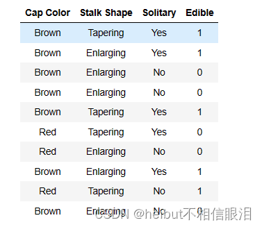
- 你有10个蘑菇的例子。对于每个示例,都有
- “三个特征”
- “Cap Color”(棕色或红色)
- “Stalk Shape”(锥形或扩大)
- “Solitary”(是或否)
- “Label Edible”
- (1表示是,0表示有毒)
3.1一个热编码数据集
为了便于实现,我们对特性进行了热编码(将它们转换为0或1值特性)
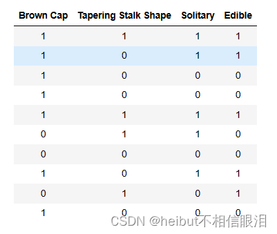
因此
- X_train包含每个示例的三个特征
- 棕色(值1表示“棕色”的菌盖颜色,0表示“红色”的菌帽颜色)
- 锥形(值1指示“锥形茎形状”,0表示茎形状“扩大”)
- 孤立(值1表明“是”,0表明“否”)
- y_train表示蘑菇是否可食用
- y=1表示可食用
- y=0表示有毒
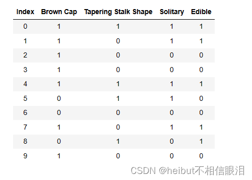
X_train = np.array([[1,1,1],[1,0,1],[1,0,0],[1,0,0],[1,1,1],[0,1,1],[0,0,0],[1,0,1],[0,1,0],[1,0,0]])
y_train = np.array([1,1,0,0,1,0,0,1,1,0])
查看变量
让我们更熟悉您的数据集。
- 一个好的开始是打印出每个变量,看看它包含什么。
下面的代码打印X_train的前几个元素和变量的类型。
print("First few elements of X_train:\n", X_train[:5])
print("Type of X_train:",type(X_train))
First few elements of X_train: [[1 1 1] [1 0 1] [1 0 0] [1 0 0] [1 1 1]] Type of X_train:
现在,让我们为y_train做同样的事情
print("First few elements of y_train:", y_train[:5])
print("Type of y_train:",type(y_train))
First few elements of y_train: [1 1 0 0 1] Type of y_train:
检查变量的维度
熟悉数据的另一种有用方法是查看其维度。
请打印X_train和y_train的形状,并查看您的数据集中有多少训练示例。
print ('The shape of X_train is:', X_train.shape)
print ('The shape of y_train is: ', y_train.shape)
print ('Number of training examples (m):', len(X_train))
The shape of X_train is: (10, 3) The shape of y_train is: (10,) Number of training examples (m): 10
4-决策树
- 回想一下,构建决策树的步骤如下:
- 从根节点的所有示例
- 开始计算所有可能特征的拆分信息增益,并选择信息增益最高的一个
- 根据所选特征拆分数据集,并创建树的左分支和右分支
- 继续重复拆分过程,直到满足停止标准。
- 在本实验室中,您将实现以下功能,使您可以使用具有最高信息增益的特征将节点拆分为左分支和右分支
- 计算节点处的熵
- 根据给定的特征将节点处的数据集拆分为左右分支
- 计算在给定特征上拆分的信息增益
- 选择最大化信息增益的特征
- 然后我们将使用您实现的辅助函数通过重复拆分过程来构建决策树,直到满足停止标准
- 对于这个实验室,我们选择的停止标准是将最大深度设置为2
4.1计算熵
首先,您将编写一个名为compute_entropy的辅助函数,用于计算节点处的熵(杂质的度量)。
- 该函数接受一个numpy数组(y),该数组指示该节点中的示例是可食用的(1)还是有毒的(0)
完成下面的compute_entropy()函数以:
-
计算𝑝1,这是可食用的例子的分数(即y中的值=1)。
-
然后熵计算为
𝐻(𝑝1)=−𝑝1*log2(𝑝1)−(1−𝑝1)*log2(1−𝑝1)
-
注:
- 对数以基数2计算
- 出于实现目的,0log2(0)=0,也就是说,如果p_1=0或p_1=1,则将熵设置为0。
- 确保检查节点处的数据是否为空(即len(y)!=0). 如果是,则返回0
练习1
请按照前面的说明完成compute_entropy()函数。
如果遇到问题,可以查看下面单元格后面的提示,以帮助您实现。
# UNQ_C1 # GRADED FUNCTION: compute_entropy def compute_entropy(y): """ Computes the entropy for Args: y (ndarray): Numpy array indicating whether each example at a node is edible (`1`) or poisonous (`0`) Returns: entropy (float): Entropy at that node """ # You need to return the following variables correctly entropy = 0. ### START CODE HERE ### if len(y) != 0: # Your code here to calculate the fraction of edible examples (i.e with value = 1 in y) p1 = len(y[y == 1])/len(y) # For p1 = 0 and 1, set the entropy to 0 (to handle 0log0) if p1 != 0 and p1 != 1: # Your code here to calculate the entropy using the formula provided above entropy = -p1 * np.log2(p1) - (1 - p1) * np.log2(1 - p1) else: entropy = 0. ### END CODE HERE ### return entropy您可以通过运行以下测试代码来检查您的实现是否正确:
# Compute entropy at the root node (i.e. with all examples)
# Since we have 5 edible and 5 non-edible mushrooms, the entropy should be 1"
print("Entropy at root node: ", compute_entropy(y_train))
# UNIT TESTS
compute_entropy_test(compute_entropy)
Entropy at root node: 1.0 All tests passed.
Expected Output:
Entropy at root node: 1.0
4.2分割数据集
接下来,您将编写一个名为Split_dataset的辅助函数,该函数接收节点上的数据和要分割的特性,并将其分割为左右分支。稍后在实验室中,您将实现代码来计算拆分的效果。
- 该函数接收训练数据、该节点的数据点索引列表以及要拆分的特征。
- 它对数据进行拆分,并返回左分支和右分支处的索引子集。
- 例如,假设我们从根节点开始(因此node_indices=[0,1,2,3,4,5,6,7,8,9]),然后我们选择在特征0上进行拆分,即示例是否有棕色帽。
- 函数的输出为,left_indices=[0,1,2,3,4,7,9],right_indices=[5,6,8]
练习2
请完成下面显示的split_dataset()函数
- 对于node_indices中的每个索引
- 如果该功能的索引处的X值为1,则将索引添加到left_indices
- 如果该功能索引处的X值为0,则将该索引添加到right_indices。
如果遇到问题,可以查看下面单元格后的提示,以帮助您实现。
# UNQ_C2 # GRADED FUNCTION: split_dataset def split_dataset(X, node_indices, feature): """ Splits the data at the given node into left and right branches Args: X (ndarray): Data matrix of shape(n_samples, n_features) node_indices (ndarray): List containing the active indices. I.e, the samples being considered at this step. feature (int): Index of feature to split on Returns: left_indices (ndarray): Indices with feature value == 1 right_indices (ndarray): Indices with feature value == 0 """ # You need to return the following variables correctly left_indices = [] right_indices = [] ### START CODE HERE ### for i in node_indices: if X[i][feature]==1: left_indices.append(i) else : right_indices.append(i) ### END CODE HERE ### return left_indices, right_indices现在,让我们使用下面的代码块来检查您的实现。让我们试着在根节点上拆分数据集,它包含了我们上面讨论过的特征0(Brown Cap)的所有示例
root_indices = [0, 1, 2, 3, 4, 5, 6, 7, 8, 9]
# Feel free to play around with these variables
# The dataset only has three features, so this value can be 0 (Brown Cap), 1 (Tapering Stalk Shape) or 2 (Solitary)
feature = 0
left_indices, right_indices = split_dataset(X_train, root_indices, feature)
print("Left indices: ", left_indices)
print("Right indices: ", right_indices)
# UNIT TESTS
split_dataset_test(split_dataset)
Left indices: [0, 1, 2, 3, 4, 7, 9] Right indices: [5, 6, 8] All tests passed.
Expected Output:
Left indices: [0, 1, 2, 3, 4, 7, 9]
Right indices: [5, 6, 8]
4.3计算信息增益
接下来,您将编写一个名为information_gain的函数,该函数接收训练数据、节点处的索引和要拆分的特征,并返回拆分后的信息增益。
练习3
请完成下面显示的compute_information_gain()函数进行计算
Information Gain=𝐻(𝑝1^node)−(𝑤^left𝐻(𝑝1^left)+𝑤^right𝐻(𝑝1^right)
- 𝐻(𝑝1^node)是节点处的熵
- 𝐻(𝑝1^left) 和 𝐻(𝑝1^right)左右分支的熵是分裂产生的
- w^left和w^right分别是左分支和右分支的示例比例
注:
- 您可以使用上面实现的compute_entropy()函数来计算熵。
- 我们提供了一些入门代码,它使用上面实施的split_dataset()函数分割数据集。
如果您遇到问题,可以查看下面单元格后面的提示,以帮助您实现。
# UNQ_C3
# GRADED FUNCTION: compute_information_gain
def compute_information_gain(X, y, node_indices, feature):

    """
    Compute the information of splitting the node on a given feature

    Args:
        X (ndarray):            Data matrix of shape(n_samples, n_features)
        y (array like):         list or ndarray with n_samples containing the target variable
        node_indices (ndarray): List containing the active indices. I.e, the samples being considered in this step.

    Returns:
        cost (float):        Cost computed

    """
    # Split dataset
    left_indices, right_indices = split_dataset(X, node_indices, feature)

    # Some useful variables
    X_node, y_node = X[node_indices], y[node_indices]
    X_left, y_left = X[left_indices], y[left_indices]
    X_right, y_right = X[right_indices], y[right_indices]

    # You need to return the following variables correctly
    information_gain = 0

    ### START CODE HERE ###

    node_entropy=compute_entropy(y_node)
    left_entropy=compute_entropy(y_left)
    right_entropy=compute_entropy(y_right)

    # Weights
    w_left = len(X_left) / len(X_node)
    w_right = len(X_right) / len(X_node)

    #Weighted entropy
    information_gain=node_entropy-(w_left*left_entropy+w_right*right_entropy)
    #Information gain

    ### END CODE HERE ###

    return information_gain
现在,您可以使用下面的单元格来检查您的实现,并计算在每个featue上拆分所获得的信息
info_gain0 = compute_information_gain(X_train, y_train, root_indices, feature=0)
print("Information Gain from splitting the root on brown cap: ", info_gain0)

info_gain1 = compute_information_gain(X_train, y_train, root_indices, feature=1)
print("Information Gain from splitting the root on tapering stalk shape: ", info_gain1)
info_gain2 = compute_information_gain(X_train, y_train, root_indices, feature=2)
print("Information Gain from splitting the root on solitary: ", info_gain2)
# UNIT TESTS
compute_information_gain_test(compute_information_gain)
Information Gain from splitting the root on brown cap: 0.034851554559677034 Information Gain from splitting the root on tapering stalk shape: 0.12451124978365313 Information Gain from splitting the root on solitary: 0.2780719051126377 All tests passed.
Expected Output:
Information Gain from splitting the root on brown cap: 0.034851554559677034
Information Gain from splitting the root on tapering stalk shape: 0.12451124978365313
Information Gain from splitting the root on solitary: 0.2780719051126377
在根节点的“孤立”(特征=2)上进行拆分可以获得最大的信息增益。因此,它是在根节点进行拆分的最佳功能。
4.4获得最佳分割
现在让我们编写一个函数,通过像上面所做的那样计算每个特征的信息增益,并返回提供最大信息增益的特征,来获得要分割的最佳特征
练习4
请完成下面显示的get_best_split()函数。
- 该函数接收训练数据,以及该节点的数据点索引。
- 函数的输出提供最大信息增益的功能。
- 您可以使用compute_information_gain()函数迭代功能并计算每个功能的信息。如果您遇到问题,可以查看下面单元格后的提示,以帮助您实现。
#123
def get_best_split(X, y, node_indices):
    # Some useful variables
    num_features = X.shape[1]
    # You need to return the following variables correctly
    best_feature = -1
    ### START CODE HERE ###
    max_info_gain = 0
    # Iterate through all features
    for feature in range(num_features):

        # Your code here to compute the information gain from splitting on this feature
        info_gain = compute_information_gain(X, y, node_indices, feature)

        # If the information gain is larger than the max seen so far
        if info_gain > max_info_gain:
            # Your code here to set the max_info_gain and best_feature
            max_info_gain = info_gain
            best_feature = feature
    ### END CODE HERE ##
    return best_feature
feature (int): Index of feature to split on
现在,让我们使用下面的单元格检查您的函数的实现情况。
best_feature = get_best_split(X_train, y_train, root_indices)
print("Best feature to split on: %d" % best_feature)
# UNIT TESTS
get_best_split_test(get_best_split)
Best feature to split on: 2 All tests passed.
正如我们在上面看到的,函数返回在根节点上分割的最佳特征是特征2(“孤立”)
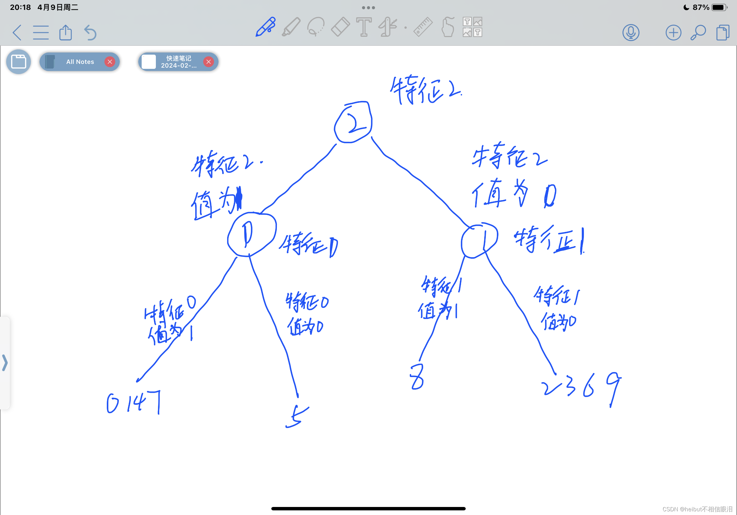
5-构建树
在本节中,我们使用您在上面实现的功能来生成决策树,方法是依次选择要拆分的最佳特征,直到达到停止标准(最大深度为2)。
您不需要为此部分实现任何内容。
# Not graded
tree = []
def build_tree_recursive(X, y, node_indices, branch_name, max_depth, current_depth):
    """
    Build a tree using the recursive algorithm that split the dataset into 2 subgroups at each node.
    This function just prints the tree.

    Args:
        X (ndarray):            Data matrix of shape(n_samples, n_features)
        y (array like):         list or ndarray with n_samples containing the target variable
        node_indices (ndarray): List containing the active indices. I.e, the samples being considered in this step.
        branch_name (string):   Name of the branch. ['Root', 'Left', 'Right']
        max_depth (int):        Max depth of the resulting tree.
        current_depth (int):    Current depth. Parameter used during recursive call.

    """
    # Maximum depth reached - stop splitting
    if current_depth == max_depth:
        formatting = " "*current_depth + "-"*current_depth
        print(formatting, "%s leaf node with indices" % branch_name, node_indices)
        return

    # Otherwise, get best split and split the data
    # Get the best feature and threshold at this node
    best_feature = get_best_split(X, y, node_indices)
    tree.append((current_depth, branch_name, best_feature, node_indices))

    formatting = "-"*current_depth
    print("%s Depth %d, %s: Split on feature: %d" % (formatting, current_depth, branch_name, best_feature))

    # Split the dataset at the best feature
    left_indices, right_indices = split_dataset(X, node_indices, best_feature)

    # continue splitting the left and the right child. Increment current depth
    build_tree_recursive(X, y, left_indices, "Left", max_depth, current_depth+1)
    build_tree_recursive(X, y, right_indices, "Right", max_depth, current_depth+1)
build_tree_recursive(X_train, y_train, root_indices, "Root", max_depth=2, current_depth=0)
 Depth 0, Root: Split on feature: 2
- Depth 1, Left: Split on feature: 0
  -- Left leaf node with indices [0, 1, 4, 7]
  -- Right leaf node with indices [5]
- Depth 1, Right: Split on feature: 1
  -- Left leaf node with indices [8]
  -- Right leaf node with indices [2, 3, 6, 9]
- 您可以使用compute_information_gain()函数迭代功能并计算每个功能的信息。如果您遇到问题,可以查看下面单元格后的提示,以帮助您实现。
- 函数的输出为,left_indices=[0,1,2,3,4,7,9],right_indices=[5,6,8]
-
- 该函数接受一个numpy数组(y),该数组指示该节点中的示例是可食用的(1)还是有毒的(0)
- 对于这个实验室,我们选择的停止标准是将最大深度设置为2
- 回想一下,构建决策树的步骤如下:
- 一个好的开始是打印出每个变量,看看它包含什么。
- X_train包含每个示例的三个特征
- (1表示是,0表示有毒)
- “三个特征”
- 你有10个蘑菇的例子。对于每个示例,都有