
1、空间滤波原理
空间滤波,就是在原图像上,用一个固定尺寸的模板去做卷积运算,得到的新图像就是滤波结果。滤波,就是过滤某种信号的意思。过滤哪种信号取决于模板设计,如果是锐化模板,处理后就保留高频信号,如果是平滑模板,处理后就保留低频信号。
(1)模板运算
图像处理中模板能够看作是n*n(n通常是奇数)的窗体。模板连续地运动于整个图像中,对模板窗体范围内的像素做相应处理。
模板运算主要分为:
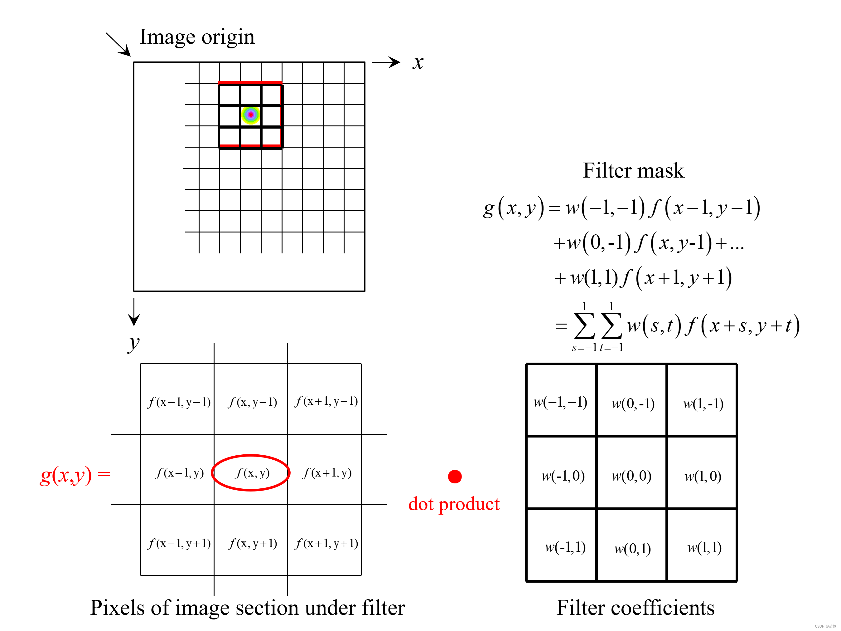
①模板卷积。模板卷积是把模板内像素的灰度值和模板中相应的灰度值相乘,求平均值赋给当前模板窗体的中心像素。作为它的灰度值;
②模板排序。模板排序是把模版内像素的灰度值排序,取某个顺序统计量作为模板中心像素灰度值。
Matlab中做模版卷积十分高效,取出模版内子矩阵和模版权重点乘求平均就可以,已图示为例,3X3的模板在图像上滑动,原图像f(x,y) 经过模板处理后变成了g(x,y)。
(2)边界处理
处理边界有非常多种做法:
①重复图像边缘上的行和列。
②卷绕输入图像(假设第一列紧接着最后一列)。
③在输入图像外部填充常数(例如零)。
④去掉不能计算的行列。仅对可计算的像素计算卷积。
(3)空间域滤波
把模板运算运用于图像的空间域增强的技术称为空间域滤波。依据滤波频率空间域滤波分为平滑滤波(减弱和去除高频分量)和锐化滤波(减弱和去除低频分量),依据滤波计算特点又分为线性滤波和非线性滤波。
因此空间域滤波可分为:
分类 线性 非线性
平滑 线性平滑 非线性平滑
锐化 线性锐化 非线性锐化
2、平滑滤波器
(1)添加噪声
噪声主要分类为两类,高斯噪声和椒盐噪声。
高斯噪声在每个像素上都会出现,赋值服从高斯分布。
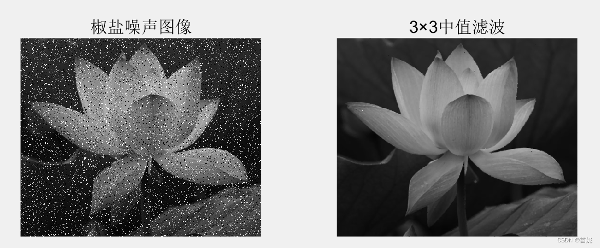
椒盐噪声出现位置随机,所以可以控制椒盐噪声的密度,椒盐噪声的幅度确定,椒噪声偏暗,盐噪声偏亮。

Image = mat2gray( imread('original_pattern.jpg') ,[0 255]);
noiseIsp=imnoise(Image,'salt & pepper',0.1);  %添加椒盐噪声,密度为0.1
imshow(noiseIsp,[0 1]); title('椒盐噪声图像');
noiseIg=imnoise(Image,'gaussian'); %添加高斯噪声,默认均值为0,方差为0.01
figure;imshow(noiseIg,[0 1]); title('高斯噪声图像');
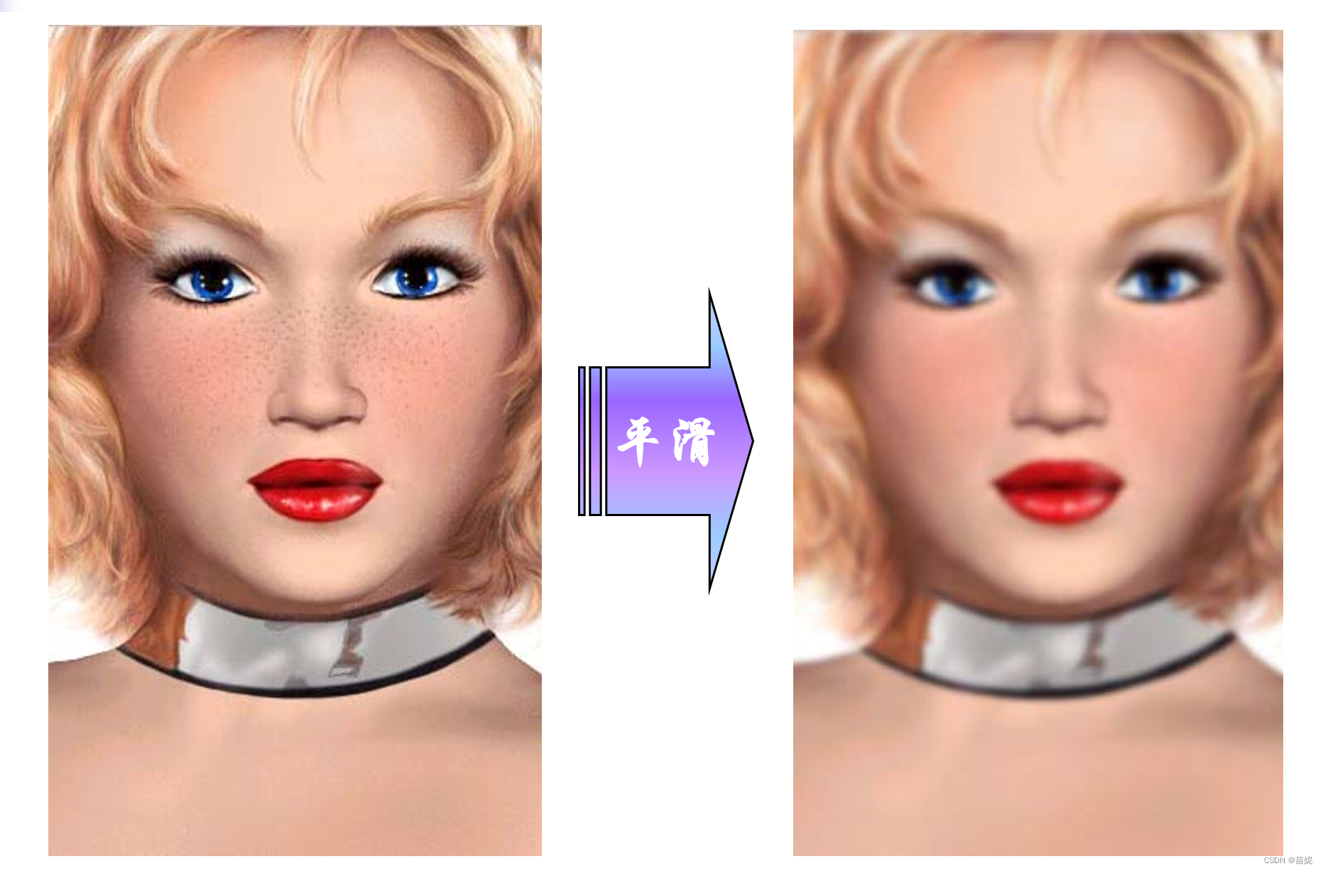
(2)平滑滤波器
平滑滤波器可以去除图像的噪声,使图像变得模糊。包括:中值滤波、均值滤波、高斯滤波。
高斯滤波、均值滤波去除高斯噪声。
 (3)均值滤波

Image=imread('Letters-a.jpg');
noiseI=imnoise(Image,'gaussian');                %添加高斯噪声
subplot(221),imshow(Image),title('原图');
subplot(222),imshow(noiseI),title('高斯噪声图像');
result1=filter2(fspecial('average',3),noiseI);                %3×3均值滤波
result2=filter2(fspecial('average',7),noiseI);                % 7×7均值滤波
subplot(223),imshow(uint8(result1)),title('3×3均值滤波');
subplot(224),imshow(uint8(result2)),title('7×7均值滤波');
(4)中值滤波
Image=rgb2gray(imread('lotus.bmp'));
noiseI=imnoise(Image,'salt & pepper',0.1);
result=medfilt2(noiseI);                                 %3×3中值滤波
subplot(121),imshow(noiseI),title('椒盐噪声图像');
subplot(122),imshow(uint8(result)),title('3×3中值滤波');
(5)自编程实现高斯滤波

Image=imread('Letters-a.jpg');
sigma1=0.6; sigma2=10; r=3;  % 高斯模板的参数
NoiseI= imnoise(Image,'gaussian'); %加噪
gausFilter1=fspecial('gaussian',[2*r+1 2*r+1],sigma1);
gausFilter2=fspecial('gaussian',[2*r+1 2*r+1],sigma2);
result1=imfilter(NoiseI,gausFilter1,'conv');
result2=imfilter(NoiseI,gausFilter2,'conv');
subplot(231);imshow(Image);title('原图');
subplot(232);imshow(NoiseI);title('高斯噪声图像');
subplot(233);imshow(result1);title('sigma1 =0.6高斯滤波');
subplot(234);imshow(result2);title('sigma2 =10高斯滤波');
%imwrite(uint8(NoiseI),'gr.bmp');
%imwrite(uint8(result1),'gr1.bmp');
%imwrite(uint8(result2),'gr2.bmp');
%编写高斯滤波函数实现
[height,width]=size(NoiseI);
for x=-r:r
    for y=-r:r
        H(x+r+1,y+r+1)=1/(2*pi*sigma1^2).*exp((-x.^2-y.^2)/(2*sigma1^2));
    end
end
H=H/sum(H(:));  %归一化高斯模板H
result3=zeros(height,width);            %滤波后图像
midimg=zeros(height+2*r,width+2*r);    %中间图像
midimg(r+1:height+r,r+1:width+r)=NoiseI;
for ai=r+1:height+r
    for aj=r+1:width+r
        temp_row=ai-r;
        temp_col=aj-r;
        temp=0;
        for bi=1:2*r+1
            for bj=1:2*r+1
                temp= temp+(midimg(temp_row+bi-1,temp_col+bj-1)*H(bi,bj));
            end
        end
       result3(temp_row,temp_col)=temp;
    end
end
subplot(235);imshow(uint8(result3));title('myself高斯滤波');
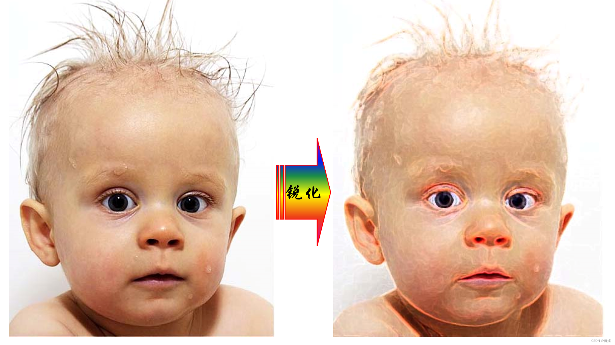
3、锐化滤波器
(1)梯度算子
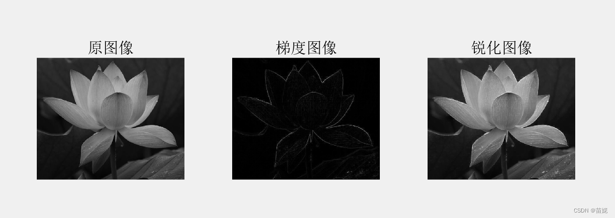
Image=im2double(rgb2gray(imread('lotus.jpg')));
subplot(131),imshow(Image),title('原图像');
[h,w]=size(Image);
edgeImage=zeros(h,w);
for x=1:w-1
    for y=1:h-1
        edgeImage(y,x)=abs(Image(y,x+1)-Image(y,x))+abs(Image(y+1,x)-Image(y,x));
    end
end
subplot(132),imshow(edgeImage),title('梯度图像');
sharpImage=Image+edgeImage;
subplot(133),imshow(sharpImage),title('锐化图像');
(2)Robert算子

Image=im2double(rgb2gray(imread('lotus.jpg')));
subplot(221),imshow(Image),title('原图像');
BW= edge(Image,'roberts');
subplot(222),imshow(BW),title('边缘检测');
H1=[1 0; 0 -1];
H2=[0 1;-1 0];
R1=imfilter(Image,H1);
R2=imfilter(Image,H2);
edgeImage=abs(R1)+abs(R2);
subplot(223),imshow(edgeImage),title('Robert梯度图像');
sharpImage=Image+edgeImage;
subplot(224),imshow(sharpImage),title('Robert锐化图像');
(3)Sobel算子

Image=im2double(rgb2gray(imread('lotus.jpg')));
subplot(221),imshow(Image),title('原图像');
BW= edge(Image,'sobel');
subplot(222),imshow(BW),title('边缘检测');
H1=[-1 -2 -1;0 0 0;1 2 1];
H2=[-1 0 1;-2 0 2;-1 0 1];
R1=imfilter(Image,H1);
R2=imfilter(Image,H2);
edgeImage=abs(R1)+abs(R2);
subplot(223),imshow(edgeImage),title('Sobel梯度图像');
sharpImage=Image+edgeImage;
subplot(224),imshow(sharpImage),title('Sobel锐化图像');
(4)多个模板边缘检测

clear,clc,close all;
Image=im2double(rgb2gray(imread('lotus.jpg')));
H1=[-1 -1 -1;0 0 0;1 1 1];
H2=[0 -1 -1;1 0 -1; 1 1 0];
H3=[1 0 -1;1 0 -1;1 0 -1];
H4=[1 1 0;1 0 -1;0 -1 -1];
H5=[1 1 1;0 0 0;-1 -1 -1];
H6=[0 1 1;-1 0 1;-1 -1 0];
H7=[-1 0 1;-1 0 1;-1 0 1];
H8=[-1 -1 0;-1 0 1;0 1 1];
R1=imfilter(Image,H1);
R2=imfilter(Image,H2);
R3=imfilter(Image,H3);
R4=imfilter(Image,H4);
R5=imfilter(Image,H5);
R6=imfilter(Image,H6);
R7=imfilter(Image,H7);
R8=imfilter(Image,H8);
edgeImage1=abs(R1)+abs(R7);
sharpImage1=edgeImage1+Image;
f1=max(max(R1,R2),max(R3,R4));
f2=max(max(R5,R6),max(R7,R8));
edgeImage2=max(f1,f2);
sharpImage2=edgeImage2+Image;
subplot(221),imshow(edgeImage1),title('两个模板边缘检测');
subplot(222),imshow(edgeImage2),title('八个模板边缘检测');
subplot(223),imshow(sharpImage1),title('两个模板边缘锐化');
subplot(224),imshow(sharpImage2),title('八个模板边缘锐化');
(5)Laplacian算子
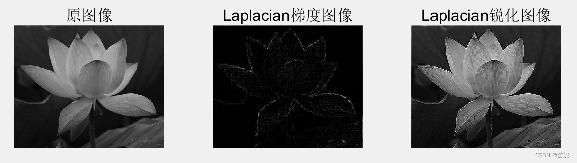
Image=im2double(rgb2gray(imread('lotus.jpg')));
subplot(131),imshow(Image),title('原图像');
H=fspecial('laplacian',0);
R=imfilter(Image,H);
edgeImage=abs(R);
subplot(132),imshow(edgeImage),title('Laplacian梯度图像');
H1=[0 -1 0;-1 5 -1;0 -1 0];
sharpImage=imfilter(Image,H1);
subplot(133),imshow(sharpImage),title('Laplacian锐化图像');