格拉姆角场

格拉姆角场学习GAF官方文档

格拉姆角场能够将时间序列数据转换为图像数据，既能保留信号完整的信息，也保持着信号对于时间的依赖性。信号数据转换为图像数据后就可以充分利用CNN在图像分类识别上的优势，进行建模 。

Document:

为每个(x_i, x_j)创建一个时间相关性矩阵。首先，它以-1

[外链图片转存失败,源站可能有防盗链机制,建议将图片保存下来直接上传(img-mIHtqGZ3-1678874178580)(null)]

格拉姆矩阵：假设有一个向量V，Gram矩阵就是来自V的每一对向量的内积矩阵。

• 通过取每个 M 点的平均值来聚合时间序列以减小大小。此步骤使用分段聚合近似PAA ( Piecewise Aggregation Approximation / PAA)。
• 区间[0,1]中的缩放值。
• 通过将时间戳作为半径和缩放值的反余弦（arccosine）来生成极坐标。这杨可以提供角度的值。
• 生成GASF / GADF。在这一步中，将每对值相加（相减），然后取余弦值后进行求和汇总
• 
• 通过取时间序列值的余弦倒数来计算 A 和 B（实际上是在 PAA 和缩放之后的值上）

  代码实例

  1. 分段聚合近似PAA

  # Author: Johann Faouzi 
  # License: BSD-3-Clause
  import numpy as np
  import matplotlib.pyplot as plt
  from pyts.approximation import PiecewiseAggregateApproximation
  # Parameters
  n_samples, n_timestamps = 100, 48
  # Toy dataset
  rng = np.random.RandomState(41)
  X = rng.randn(n_samples, n_timestamps)
  # PAA transformation
  window_size = 6
  paa = PiecewiseAggregateApproximation(window_size=window_size)
  X_paa = paa.transform(X)
  # Show the results for the first time series
  plt.figure(figsize=(6, 4))
  plt.plot(X[0], 'o--', ms=4, label='Original')
  plt.plot(np.arange(window_size // 2,
                     n_timestamps + window_size // 2,
                     window_size), X_paa[0], 'o--', ms=4, label='PAA')
  plt.vlines(np.arange(0, n_timestamps, window_size) - 0.5,
             X[0].min(), X[0].max(), color='g', linestyles='--', linewidth=0.5)
  plt.legend(loc='best', fontsize=10)
  plt.xlabel('Time', fontsize=12)
  plt.title('Piecewise Aggregate Approximation', fontsize=16)
  plt.show()
  

  Gramian Angular Field（时间序列转图像的过程）

  # python 示例
  # 导入需要的包
  from pyts.approximation import PiecewiseAggregateApproximation
  from pyts.preprocessing import MinMaxScaler
  import numpy as np
  import matplotlib.pyplot as plt
  # 生成一些demo数据
  X = [[1,2,3,4,5,6,7,8],[23,56,52,46,34,67,70,60]]
  plt.plot(X[0],X[1])
  plt.title(‘Time series’)
  plt.xlabel(‘timestamp’)
  plt.ylabel(‘value’)
  plt.show()
  # 分段聚合逼近和缩放
  # PAA
  transformer = PiecewiseAggregateApproximation(window_size=2)
  result = transformer.transform(X)
  # Scaling in interval [0,1]
  scaler = MinMaxScaler()
  scaled_X = scaler.transform(result)
  plt.plot(scaled_X[0,:],scaled_X[1,:])
  plt.title(‘After scaling’)
  plt.xlabel(‘timestamp’)
  plt.ylabel(‘value’)
  plt.show()
  # 转换成极坐标
  arccos_X = np.arccos(scaled_X[1,:])
  fig, ax = plt.subplots(subplot_kw={‘projection’: ‘polar’})
  ax.plot(result[0,:], arccos_X)
  ax.set_rmax(2)
  ax.set_rticks([0.5, 1, 1.5, 2]) # Less radial ticks
  ax.set_rlabel_position(-22.5) # Move radial labels away from plotted line
  ax.grid(True)
  ax.set_title(“Polar coordinates”, va=’bottom’)
  plt.show()
  # Gramina angular summation fields
  field = [a+b for a in arccos_X for b in arccos_X]
  gram = np.cos(field).reshape(-1,4)
  plt.imshow(gram)
  

  参考文献：

  《Encoding Time Series as Images for Visual Inspection and Classification Using Tiled Convolutional Neural Networks》 janurary,2015

  Gramian Angular Field

  给定一个时间序列X，将其缩放到[-1,1]，

  

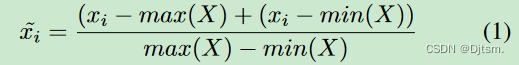
  然后再在极坐标系中表示该时间序列（通过将value编码为angular cosine，将时间戳编码为radius，

  

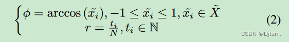
  ti是时间戳，N是正则化极坐标系统跨度的常数因子。这种基于极坐标的表示方法是理解时间序列的一种新方法。随着时间的增加，相应的值在跨越圆上的不同角度点之间扭曲，就像水荡漾一样。

  

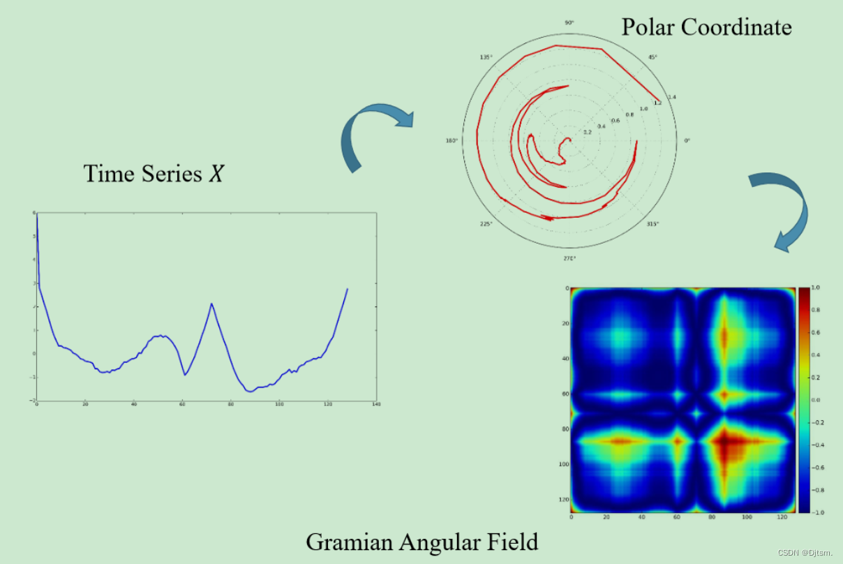
  • 等式2的编码映射有两个重要的性质。首先，当φ∈[0，π]时，当cos（φ）单调时，它是双射的。给定一个时间序列，所提出的映射在极坐标系中产生且仅一个具有唯一反函数的结果。
  • 它提供了一种保持时间依赖性的方法，因为随着位置从左上角移动到右下角，时间会增加。GAF包含时间相关性，因为G（i，ji j=k）通过相对于时间间隔k的方向叠加来表示相对相关性

    Question：当编码为反函数值时，-1和1怎么确定呢？value都是正的时，对应两个角度（在 0 0 0到 2 π 2\pi 2π上）。。。怎么选