
机器学习之Matlab代码--基于VMD与SSA优化lssvm的功率预测(多变量)(七)
- 代码
- 数据
- 结果
代码
先对外层代码的揭露,包括:顺序而下
1、
function s = Bounds( s, Lb, Ub)
% Apply the lower bound vector
temp = s;
I = temp  Ub;
temp(J) = Ub(J);
% Update this new move
s = temp;
2、
function [in,out]=data_process(data,num)
% 采用1-num的各种值为输入 第num+1的功率作为输出
n=length(data)-num;
for i=1:n
    x(i,:,:)=data(i:i+num,:);
end
in=x(1:end-1,:);
out=x(2:end,end);%功率是最后一列
3、
function y=fitness(x,train_x,train_y,test_x,test_y,typeID,kernelnamescell)
gam=x(1);
sig2=x(2);
model=initlssvm(train_x,train_y,typeID,gam,sig2,kernelnamescell);
model=trainlssvm(model);
y_pre_test=simlssvm(model,test_x);
y=mse(test_y-y_pre_test);
4、
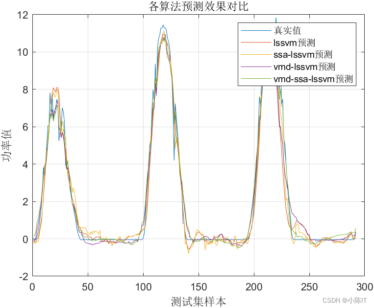
clc;clear;close all
%%
lssvm=load('lssvm.mat');
ssa_lssvm=load('ssa_lssvm.mat');
vmd_lssvm=load('vmd_lssvm.mat');
vmd_ssa_lssvm=load('vmd_ssa_lssvm.mat');
disp('结果分析-lssvm')
result(lssvm.true_value,lssvm.predict_value)
fprintf('\n')
disp('结果分析-ssa-lssvm')
result(ssa_lssvm.true_value,ssa_lssvm.predict_value)
fprintf('\n')
disp('结果分析-vmd-lssvm')
result(vmd_lssvm.true_value,vmd_lssvm.predict_value)
fprintf('\n')
disp('结果分析-vmd-ssa-lssvm')
result(vmd_ssa_lssvm.true_value,vmd_ssa_lssvm.predict_value)
figure
plot(lssvm.true_value)
hold on;grid on
plot(lssvm.predict_value)
plot(ssa_lssvm.predict_value)
plot(vmd_lssvm.predict_value)
plot(vmd_ssa_lssvm.predict_value)
legend('真实值','lssvm预测','ssa-lssvm预测','vmd-lssvm预测','vmd-ssa-lssvm预测')
title('各算法预测效果对比')
ylabel('功率值')
xlabel('测试集样本')
5、
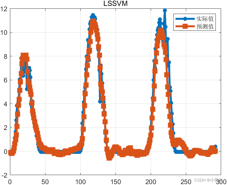
%% 其他数据与功率数据一起作为输入,参看data_process.m
clc;clear;close all
addpath(genpath('LSSVMlabv1_8'));
%%
data=xlsread('预测数据.xls','B2:K1000');
[x,y]=data_process(data,24);%前24个时刻 预测下一个时刻
%归一化
[xs,mappingx]=mapminmax(x',0,1);x=xs';
[ys,mappingy]=mapminmax(y',0,1);y=ys';
%划分数据
n=size(x,1);
m=round(n*0.7);%前70%训练,对最后30%进行预测
train_x=x(1:m,:);
test_x=x(m+1:end,:);
train_y=y(1:m,:);
test_y=y(m+1:end,:);
%% lssvm 参数
gam=10;
sig2=1000;
typeID='function estimation';
kernelnamescell='RBF_kernel';
model=initlssvm(train_x,train_y,typeID,gam,sig2,kernelnamescell);
model=trainlssvm(model);
y_pre_test=simlssvm(model,test_x);
% 反归一化
predict_value=mapminmax('reverse',y_pre_test',mappingy);
true_value=mapminmax('reverse',test_y',mappingy);
save lssvm predict_value true_value
disp('结果分析')
rmse=sqrt(mean((true_value-predict_value).^2));
disp(['根均方差(RMSE):',num2str(rmse)])
mae=mean(abs(true_value-predict_value));
disp(['平均绝对误差(MAE):',num2str(mae)])
mape=mean(abs(true_value-predict_value)/true_value);
disp(['平均相对百分误差(MAPE):',num2str(mape*100),'%'])
fprintf('\n')
figure
plot(true_value,'-*','linewidth',3)
hold on
plot(predict_value,'-s','linewidth',3)
legend('实际值','预测值')
grid on
title('LSSVM')
6、
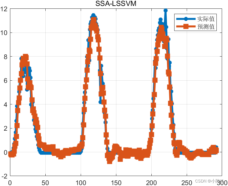
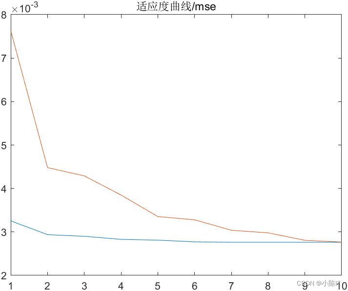
clc;clear;close all;format compact
addpath(genpath('LSSVMlabv1_8'));
%%
data=xlsread('预测数据.xls','B2:K1000');
[x,y]=data_process(data,24);%前24个时刻 预测下一个时刻
%归一化
[xs,mappingx]=mapminmax(x',0,1);x=xs';
[ys,mappingy]=mapminmax(y',0,1);y=ys';
%划分数据
n=size(x,1);
m=round(n*0.7);%前70%训练,对最后30%进行预测
train_x=x(1:m,:);
test_x=x(m+1:end,:);
train_y=y(1:m,:);
test_y=y(m+1:end,:);
%% ssa优化lssvm 参数
typeID='function estimation';
kernelnamescell='RBF_kernel';
[x,trace]=ssa_lssvm(typeID,kernelnamescell,train_x,train_y,test_x,test_y);
figure;plot(trace);title('适应度曲线/mse')
%% 利用寻优得到的参数重新训练lssvm
disp('寻优得到的参数分别是:')
gam=x(1)
sig2=x(2)
model=initlssvm(train_x,train_y,typeID,gam,sig2,kernelnamescell);
model=trainlssvm(model);
y_pre_test=simlssvm(model,test_x);
% 反归一化
predict_value=mapminmax('reverse',y_pre_test',mappingy);
true_value=mapminmax('reverse',test_y',mappingy);
save ssa_lssvm predict_value true_value
disp('结果分析')
rmse=sqrt(mean((true_value-predict_value).^2));
disp(['根均方差(RMSE):',num2str(rmse)])
mae=mean(abs(true_value-predict_value));
disp(['平均绝对误差(MAE):',num2str(mae)])
mape=mean(abs(true_value-predict_value)/true_value);
disp(['平均相对百分误差(MAPE):',num2str(mape*100),'%'])

fprintf('\n')
figure
plot(true_value,'-*','linewidth',3)
hold on
plot(predict_value,'-s','linewidth',3)
legend('实际值','预测值')
grid on
title('SSA-LSSVM')
7、
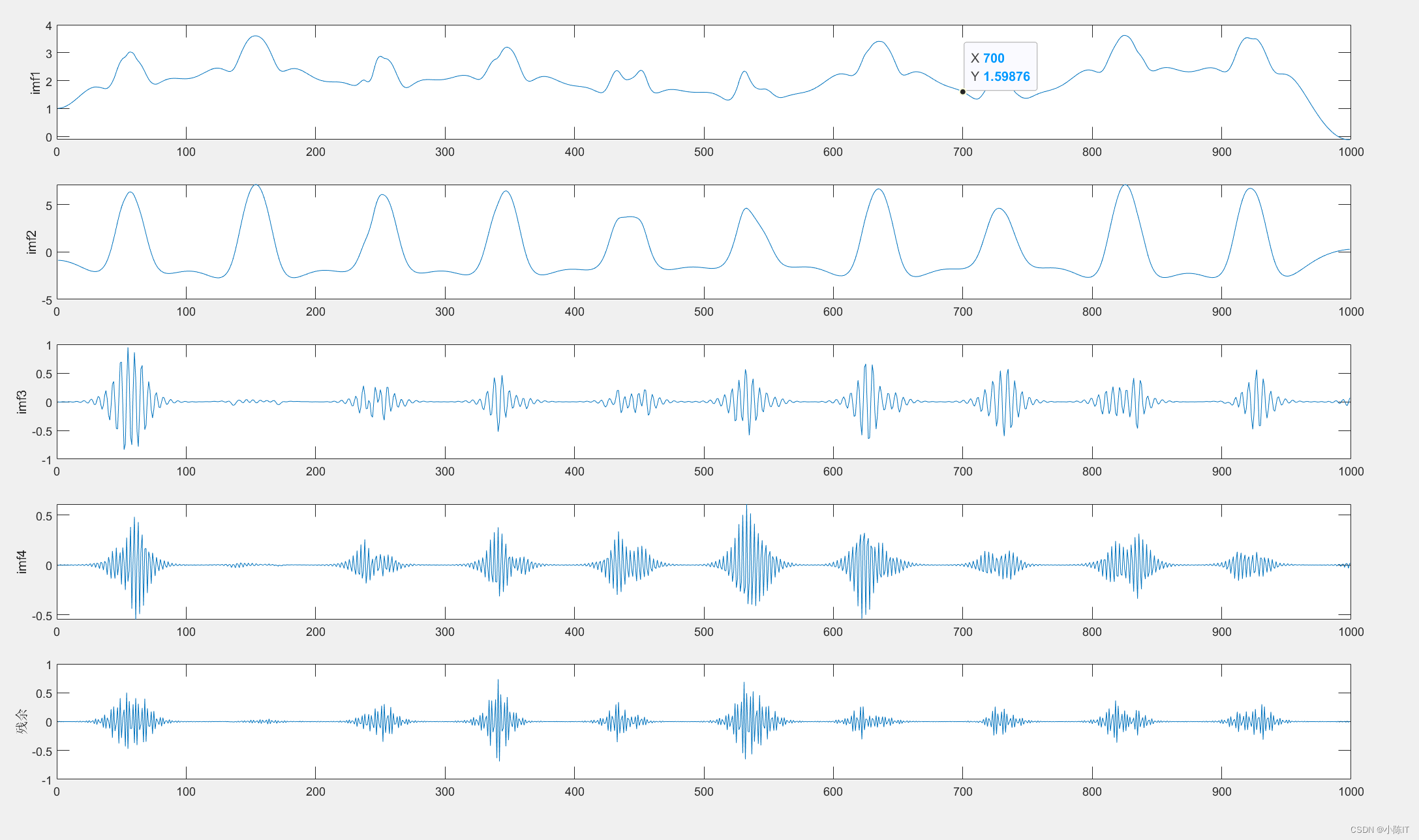
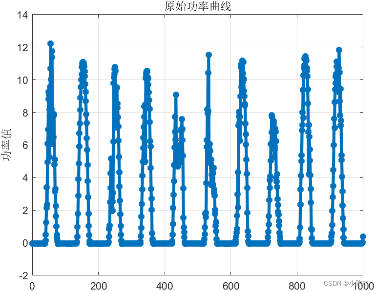
clc;clear;format compact;close all;tic
rng('default')
%% 数据预处理
data=xlsread('预测数据.xls','B2:K1000');
figure;plot(data(:,end),'-*','linewidth',3);title('原始功率曲线');grid on;ylabel('功率值')
alpha = 2000;        % moderate bandwidth constraint
tau = 0;            % noise-tolerance (no strict fidelity enforcement)
K = 5;              % 3 modes
DC = 0;             % no DC part imposed
init = 1;           % initialize omegas uniformly
tol = 1e-7;
[imf, u_hat, omega] = VMD(data(:,end), alpha, tau, K, DC, init, tol);
figure
for i =1:size(imf,1)
    subplot(size(imf,1),1,i)
    plot(imf(i,:))
    ylabel(['imf',num2str(i)])
end
ylabel('残余')
suptitle('VMD')
c=size(imf,1);
pre_result=[];
true_result=[];
%% 对每个分量建模
for i=1:c
disp(['对第',num2str(i),'个分量建模'])
[x,y]=data_process([data(:,1:end-1) imf(i,:)'],24);%每个序列和原始的几列数据合并 然后划分
%归一化
[xs,mappingx]=mapminmax(x',0,1);x=xs';
[ys,mappingy]=mapminmax(y',0,1);y=ys';
%划分数据
n=size(x,1);
m=round(n*0.7);%前70%训练,对最后30%进行预测
train_x=x(1:m,:);
test_x=x(m+1:end,:);
train_y=y(1:m,:);
test_y=y(m+1:end,:);
%%
gam=100;
sig2=1000;
typeID='function estimation';
kernelnamescell='RBF_kernel';
model=initlssvm(train_x,train_y,typeID,gam,sig2,kernelnamescell);
model=trainlssvm(model);
pred=simlssvm(model,test_x);
pre_value=mapminmax('reverse',pred',mappingy);
true_value=mapminmax('reverse',test_y',mappingy);
pre_result=[pre_result;pre_value];
true_result=[true_result;true_value];
end
%% 各分量预测的结果相加
true_value=sum(true_result);
predict_value=sum(pre_result);
save vmd_lssvm predict_value true_value
%%
load vmd_lssvm
disp('结果分析')
rmse=sqrt(mean((true_value-predict_value).^2));
disp(['根均方差(RMSE):',num2str(rmse)])
mae=mean(abs(true_value-predict_value));
disp(['平均绝对误差(MAE):',num2str(mae)])
mape=mean(abs(true_value-predict_value)/true_value);
disp(['平均相对百分误差(MAPE):',num2str(mape*100),'%'])
fprintf('\n')
figure
plot(true_value,'-*','linewidth',3)
hold on
plot(predict_value,'-s','linewidth',3)
legend('实际值','预测值')
grid on
title('VMD-LSSVM')
8、
clc;clear;format compact;close all;tic
rng('default')
%% 数据预处理
data=xlsread('预测数据.xls','B2:K1000');
figure;plot(data(:,end),'-*','linewidth',3);title('原始功率曲线');grid on;ylabel('功率值')
alpha = 2000;        % moderate bandwidth constraint
tau = 0;            % noise-tolerance (no strict fidelity enforcement)
K = 5;              % 3 modes
DC = 0;             % no DC part imposed
init = 1;           % initialize omegas uniformly
tol = 1e-7;
[imf, u_hat, omega] = VMD(data(:,end), alpha, tau, K, DC, init, tol);
figure
for i =1:size(imf,1)
    subplot(size(imf,1),1,i)
    plot(imf(i,:))
    ylabel(['imf',num2str(i)])
end
ylabel('残余')
suptitle('VMD')
c=size(imf,1);
pre_result=[];
true_result=[];
%% 对每个分量建模
for i=1:c
disp(['对第',num2str(i),'个分量建模'])
[x,y]=data_process([data(:,1:end-1) imf(i,:)'],24);
%归一化
[xs,mappingx]=mapminmax(x',0,1);x=xs';
[ys,mappingy]=mapminmax(y',0,1);y=ys';
%划分数据
n=size(x,1);
m=round(n*0.7);%前70%训练,对最后30%进行预测
train_x=x(1:m,:);
test_x=x(m+1:end,:);
train_y=y(1:m,:);
test_y=y(m+1:end,:);
%%
typeID='function estimation';
kernelnamescell='RBF_kernel';
[x,trace]=ssa_lssvm(typeID,kernelnamescell,train_x,train_y,test_x,test_y);
gam=x(1);
sig2=x(2);
model=initlssvm(train_x,train_y,typeID,gam,sig2,kernelnamescell);
model=trainlssvm(model);
pred=simlssvm(model,test_x);
pre_value=mapminmax('reverse',pred',mappingy);
true_value=mapminmax('reverse',test_y',mappingy);
pre_result=[pre_result;pre_value];
true_result=[true_result;true_value];
end
%% 各分量预测的结果相加
true_value=sum(true_result);
predict_value=sum(pre_result);
save vmd_ssa_lssvm predict_value true_value
%%
load vmd_ssa_lssvm
disp('结果分析')
rmse=sqrt(mean((true_value-predict_value).^2));
disp(['根均方差(RMSE):',num2str(rmse)])
mae=mean(abs(true_value-predict_value));
disp(['平均绝对误差(MAE):',num2str(mae)])
mape=mean(abs(true_value-predict_value)/true_value);
disp(['平均相对百分误差(MAPE):',num2str(mape*100),'%'])
fprintf('\n')
figure
plot(true_value,'-*','linewidth',3)
hold on
plot(predict_value,'-s','linewidth',3)
legend('实际值','预测值')
grid on
title('VMD-SSA-LSSVM')
9、
clear;
close all;
clc;
format compact
addpath('vmd-verify')
data=xlsread('预测数据.xls','B2:K1000');
f=data(:,end);
% some sample parameters for VMD
alpha = 2000;        % moderate bandwidth constraint
tau = 0;            % noise-tolerance (no strict fidelity enforcement)
K = 5;              % 3 modes
DC = 0;             % no DC part imposed
init = 1;           % initialize omegas uniformly
tol = 1e-7;
%--------------- Run actual VMD code
[u, u_hat, omega] = VMD(f, alpha, tau, K, DC, init, tol);
figure
plot(f)
title('原始')
figure
for i=1:K
    subplot(K,1,i)
plot(u(i,:))
ylabel(['IMF_',num2str(i)])
end
ylabel('res')
10、
function result(true_value,predict_value)
rmse=sqrt(mean((true_value-predict_value).^2));
disp(['根均方差(RMSE):',num2str(rmse)])
mae=mean(abs(true_value-predict_value));
disp(['平均绝对误差(MAE):',num2str(mae)])
mape=mean(abs(true_value-predict_value)/true_value);
disp(['平均相对百分误差(MAPE):',num2str(mape*100),'%'])
11、
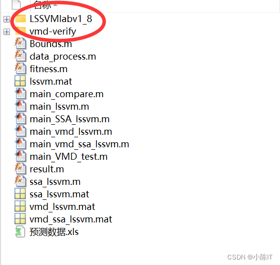
function [bestX,Convergence_curve]=ssa_lssvm(typeID,Kernel_type,inputn_train,label_train,inputn_test,label_test) %% 麻雀优化 pop=10; % 麻雀数 M=10; % Maximum numbef of iterations c=1; d=10000; dim=2; P_percent = 0.2; % The population size of producers accounts for "P_percent" percent of the total population size %%%%%%%%%%%%%%%%%%%%%%%%%%%%%%%%%%%%%%%%%%%%%%%%%%%%%% pNum = round( pop * P_percent ); % The population size of the producers lb= c.*ones( 1,dim ); % Lower limit/bounds/ a vector ub= d.*ones( 1,dim ); % Upper limit/bounds/ a vector %Initialization for i = 1 : pop x( i, : ) = lb + (ub - lb) .* rand( 1, dim ); fit( i )=fitness(x(i,:),inputn_train,label_train,inputn_test,label_test,typeID,Kernel_type); end pFit = fit; pX = x; % The individual's best position corresponding to the pFit [ fMin, bestI ] = min( fit ); % fMin denotes the global optimum fitness value bestX = x( bestI, : ); % bestX denotes the global optimum position corresponding to fMin for t = 1 : M [ ans, sortIndex ] = sort( pFit );% Sort. [fmax,B]=max( pFit ); worse= x(B,:); r2=rand(1); %%%%%%%%%%%%%5%%%%%%这一部位为发现者(探索者)的位置更新%%%%%%%%%%%%%%%%%%%%%%%%% if(r2(pop/2))%这个代表这部分麻雀处于十分饥饿的状态(因为它们的能量很低,也是是适应度值很差),需要到其它地方觅食 x( sortIndex(i ), : )=randn(1)*exp((worse-pX( sortIndex( i ), : ))/(i)^2); else%这一部分追随者是围绕最好的发现者周围进行觅食,其间也有可能发生食物的争夺,使其自己变成生产者 x( sortIndex( i ), : )=bestXX+(abs(( pX( sortIndex( i ), : )-bestXX)))*(A'*(A*A')^(-1))*ones(1,dim); end x( sortIndex( i ), : ) = Bounds( x( sortIndex( i ), : ), lb, ub );%判断边界是否超出 fit( sortIndex( i ) )=fitness(x(sortIndex( i ),:),inputn_train,label_train,inputn_test,label_test,typeID,Kernel_type); end %%%%%%%%%%%%%5%%%%%%这一部位为意识到危险(注意这里只是意识到了危险,不代表出现了真正的捕食者)的麻雀的位置更新%%%%%%%%%%%%%%%%%%%%%%%%% c=randperm(numel(sortIndex));%%%%%%%%%这个的作用是在种群中随机产生其位置(也就是这部分的麻雀位置一开始是随机的,意识到危险了要进行位置移动, %处于种群外围的麻雀向安全区域靠拢,处在种群中心的麻雀则随机行走以靠近别的麻雀) b=sortIndex(c(1:10)); for j = 1 : length(b) % Equation (5) if( pFit( sortIndex( b(j) ) )>(fMin) ) %处于种群外围的麻雀的位置改变 x( sortIndex( b(j) ), : )=bestX+(randn(1,dim)).*(abs(( pX( sortIndex( b(j) ), : ) -bestX))); else %处于种群中心的麻雀的位置改变 x( sortIndex( b(j) ), : ) =pX( sortIndex( b(j) ), : )+(2*rand(1)-1)*(abs(pX( sortIndex( b(j) ), : )-worse))/ ( pFit( sortIndex( b(j) ) )-fmax+1e-50); end x( sortIndex(b(j) ), : ) = Bounds( x( sortIndex(b(j) ), : ), lb, ub ); fit( sortIndex( b(j) ) )=fitness(x(sortIndex(b(j) ),:),inputn_train,label_train,inputn_test,label_test,typeID,Kernel_type); end for i = 1 : pop if ( fit( i )接下来是内嵌代码,就是下面两个文件夹的代码,实在是太多,想要的留言吧!
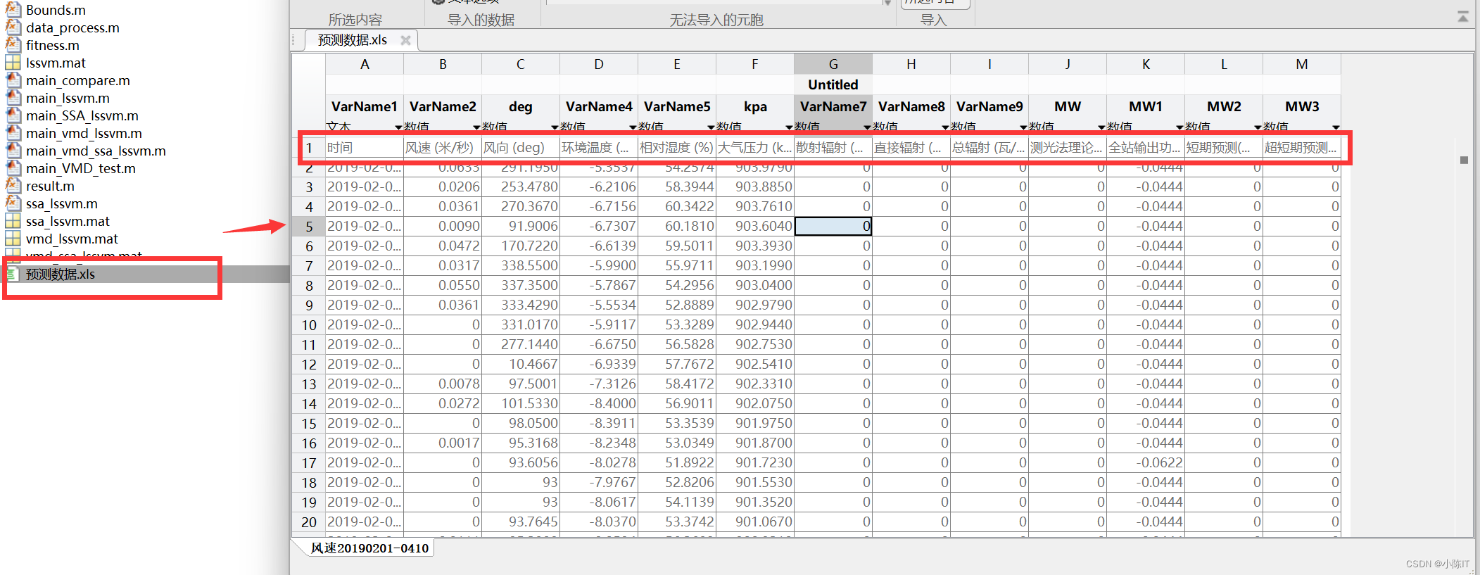
数据
数据是由时间、风速、风向等等因素组成的文件。
结果
结果图太多,就先给出这么多,如有需要代码和数据的同学请在评论区发邮箱,一般一天之内会回复,请点赞+关注谢谢!!
- 结果