Matlab 线性拟合、一维、多维度非线性拟合、多项式拟合

一、线性拟合

  线性拟合

我随便设定一个函数然后通过解方程计算出对应的系数

假设我的函数原型是

y=a*sin(0.1*x.^2+x)+b* squre(x+1)+c*x+d

clc;
clear;
x=0:0.2:10;
% 我们这里假设 a=3.2 b=0.7  c=5.0 d是一个随机
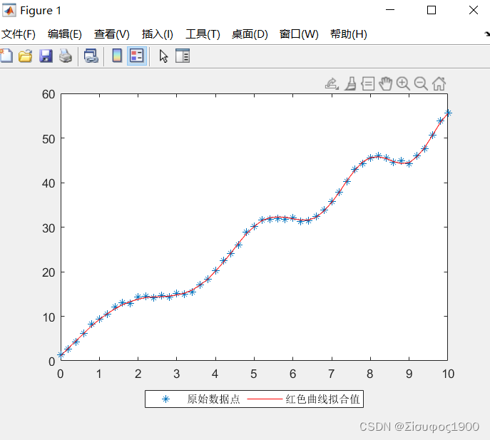
y=3.2*sin(0.1*x.^2+x)+0.7*sqrt(x+1)+5*x +rand(size(x));
plot(x,y,'*');
hold on ;
y1=sin(0.1*x.^2+x);
y2=sqrt(x+1);
y3=x;
y4=rand(size(x));
X=[y1;y2;y3;y4];%将各自的俩带入
P=X'\y'  % 通过解方程计算出4个系数
yn=P(1)*y1+P(2)*y2+P(3)*y3+P(4)*y4;  % 得到一个新的函数 计算得出的拟合Y的值 
plot(x,yn,'r');
legend('原始数据点','红色曲线拟合值','Location','southoutside','Orientation','horizontal')

 拟合系数：

clear;
clc;
close all
t=0:0.001:2*pi;%原函数
YS=sin(t);%基函数
N=21;
Yo=[];
for k=1:N
    Yn=sawtooth(k*(t+pi/2),0.5);
    Yo=[Yo,Yn'];
end
YS=YS';%拟合
a = Yo\YS;
%绘图
figure()
for k=1:N
    clf
    plot(t,Yo(:,1:k)*a(1:k,:),t,YS,'LineWidth',1)
    ylim([-1.3,1.3])
    xlim([0,6.3])
    pause(0.1)
end

二、非线性拟合

利用matlab实现非线性拟合（三维、高维、参数方程）_matlab多元非线性拟合_hyhhyh21的博客-CSDN博客

上面的这位是真正的大佬，我们都是照猫画虎的学习。

1、一维

简单的一维的拟合：

思路： 将非线性-》线性：

eg:

 将其两边都取对数

用线性的方式计算出a b 

逆变换 ，画出曲线：

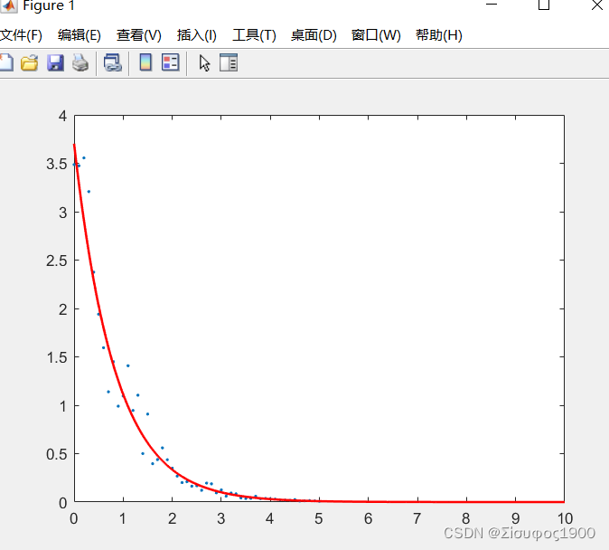
clear 
clc
close all
% 假设函数 为 y=a* exp(-bx)
x=0:0.1:5;
% 我们这里假设 a=2.4  b=1.2
a=2.4;
b=1.2;
y=a*exp(-b*x);%
y=y+1.3*y.*rand(size(y));  % 增加噪声
plot(x,y,'.');
hold on;
%Lg_y=Lg_a+b*(-x)  变成了ax+b 的形式 ，然而我们的最终的目的是通过x 来计算出a 和 b 
% 对等式的两边取对数
lg_y=log(y);
y1=ones(size(x));
y2=-x;
% 同理和上面计算线性的一杨
X=[y1;y2];
P =X'\lg_y'
% 画出拟合后的曲线
a_fit=exp(P(1));
b_fit=P(2);
x2=0:0.01:10;
plot(x2,a_fit*exp(-b_fit*x2),'-','linewidth',1.5,'color','r')

Matlab 中的非线性拟合方法

1、fit 方法

fit是最常用，最经典的方法

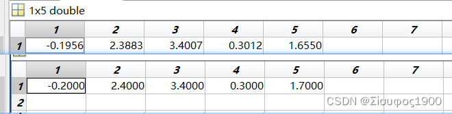
ft = fittype( 'a*x+b*sin(c*x).*exp(d*x)+e', 'independent', 'x', 'dependent', 'y' );; %函数的表达式， 
OP1 = fitoptions( 'Method', 'NonlinearLeastSquares' );% 非线性拟合方法
OP1.StartPoint = 5*rand(1,5);%初始值，越靠近真实值越好
OP1.Lower = [-2, 0, 2, 0, 0];%参数的最小边界
OP1.Upper = [1,  3, 5, 2, 3];%参数的最大边界
%   开始拟合
fitobject = fit(x',y',ft,OP1);
Fit_P=ones(size(P));
Fit_P(1)=fitobject.a;
Fit_P(2)=fitobject.b;
Fit_P(3)=fitobject.c;
Fit_P(4)=fitobject.d;
Fit_P(5)=fitobject.e;

2、nlinfit()函数 Levenberg-Marquard

L-M 非线性迭代

% 2 用nlinfit()函数 Levenberg-Marquardt 
% 定义一个函数
Func=@(P,x)( P(1)*x+P(2)*sin(P(3)*x).*exp(P(4)*x)+P(5));% 也就是说定义一个函数模型
OP2 = statset('nlinfit');% 
%  x，y  modelfun是函数模型  beta表示的是初始值 ，我这里写成最进行的那个参数   OP2  拟合的方法
beta=[-0.17 2.1  3.0  0.25  2.0];% 初始值
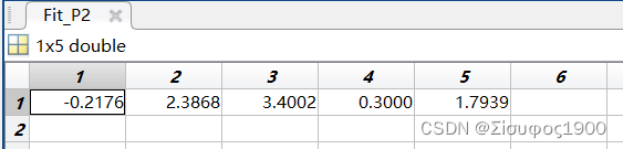
Fit_P2 = nlinfit(x,y,Func,beta,OP2);
%拟合
fit_y2 = Fit_P2(1)*x1+Fit_P2(2)*sin(Fit_P2(3)*x1).*exp(Fit_P2(4)*x1)+Fit_P2(5);;
subplot(3,2,2)
hold on;
plot(x,y,'LineStyle','none','MarkerSize',15,'Marker','.','color','k')
plot(x1,fit_y2,'-','linewidth',1.5,'color','r');
box on
%ylim(y_lim)
title('nlinfit函数')

3、信赖域法（trust region reflective）

信赖域法（trust region reflective）是通过Hessian 矩阵，逐步试探邻域内的最小化，来求解问题的。相比较之前的那些雅克比相关的方法，信赖域法会占用更多内存和速度，所以适用于中小规模的矩阵。

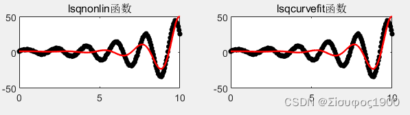
% 3 信赖区间  IsqNonLin()
func2=@(P)(P(1)*x+P(2)*sin(P(3)*x).*exp(P(4)*x)+P(5)   -y);
% lsqnonlin方法  
% 'Algorithm','trust-region-reflective'  算法是trust-region-reflective
% MaxFunctionEvaluations  MaxFunctionEvaluations可以理解为试探的次数，
%                        比如算法在一个点的四周试探了三个邻近点的值，然后确定下一步要往其中的某个点走，
%                        这个时候FunctionEvaluations对应3次，即试探了3次，而Iteration是一次，即走了一步，完成了一步迭代
% MaxIterations  最大迭代次数
OP3=optimoptions(@lsqnonlin,'Algorithm','trust-region-reflective','MaxFunctionEvaluations',1e4,'MaxIterations',1e3);
%[-2, 0, 2, 0, 0];%参数的最小边界
%[1,  3, 5, 2, 3];%参数的最大边界
lower=[-2, 0, 2, 0, 0];
up=[1,  3, 5, 2, 3];
% 计算出系数
[Fit_P3,~]=lsqnonlin(func2,beta,lower,up,OP3);
fit_y3=Fit_P3(1)*x1+Fit_P3(2)*sin(Fit_P3(3)*x1).*exp(Fit_P3(4)*x1)+Fit_P3(5);
subplot(3,2,3);
hold on
plot(x,y,'LineStyle','none','MarkerSize',15,'Marker','.','color','k')
plot(x1,fit_y3,'-','linewidth',1.5,'color','r')
hold off
box on
%ylim(y_lim)
title('lsqnonlin函数');
%4 lsqcurvefit()函数 trust-region-reflective
modelfun2 = @(p,x)(p(1)*x+p(2)*sin(p(3)*x).*exp(p(4)*x)+p(5)) ;
OP4=optimoptions('lsqcurvefit','Algorithm','trust-region-reflective','MaxFunctionEvaluations',1e4,'MaxIterations',1e3);
%[-2, 0, 2, 0, 0];%参数的最小边界
%[1,  3, 5, 2, 3];%参数的最大边界
lower=[-2, 0, 2, 0, 0];
up=[1,  3, 5, 2, 3];
% 计算出系数
%[p,~] = lsqcurvefit(modelfun,p0,x,y,[-2,0,2,0,0],[1,3,5,3,3],OP4);
[Fit_P4,~]=lsqcurvefit(modelfun2,beta,x,y,lower,up,OP4);
fit_y4=Fit_P4(1)*x1+Fit_P4(2)*sin(Fit_P4(3)*x1).*exp(Fit_P4(4)*x1)+Fit_P4(5);
subplot(3,2,4);
hold on
plot(x,y,'LineStyle','none','MarkerSize',15,'Marker','.','color','k')
plot(x1,fit_y4,'-','linewidth',1.5,'color','r')
hold off
box on
%ylim(y_lim)
title('lsqcurvefit函数');

4、fsolve()函数

默认的算法为trust-region-dogleg，属于信赖域法。

5、粒子群法

 所有代码：

clear;
close all;
clc;
% 自定义一个非线性的函数 y=a*x+b*sin(c*x).*exp(d*x)+e  那将函数
x = 0:0.05:10;
P=[-0.2 2.4  3.4  0.3 1.7];
y = P(1)*x+P(2)*sin(P(3)*x).*exp(P(4)*x)+P(5);
y=y+0.5*randn(size(x)); % 添加噪声 
figure();
% 1 .fit 函数开始拟合
ft = fittype( 'a*x+b*sin(c*x).*exp(d*x)+e', 'independent', 'x', 'dependent', 'y' );; %函数的表达式， 
OP1 = fitoptions( 'Method', 'NonlinearLeastSquares' );% 非线性拟合方法
%OP1.StartPoint = 5*rand(1,5);%初始值，越靠近真实值越好
OP1.StartPoint = [-0.17 2.1  3.0  0.25  2.0];
OP1.Lower = [-2, 0, 2, 0, 0];%参数的最小边界
OP1.Upper = [1,  3, 5, 2, 3];%参数的最大边界
%   开始拟合
fitobject = fit(x',y',ft,OP1);
Fit_P=ones(size(P));
Fit_P(1)=fitobject.a;
Fit_P(2)=fitobject.b;
Fit_P(3)=fitobject.c;
Fit_P(4)=fitobject.d;
Fit_P(5)=fitobject.e;
%plot(x,y,'.');
% 开始计算拟合后的y 
x1 = 0:0.01:10;
fit_y1 = Fit_P(1)*x1+Fit_P(2)*sin(Fit_P(3)*x1).*exp(Fit_P(4)*x1)+Fit_P(5);
subplot(3,2,1)
hold on
plot(x,y,'LineStyle','none','MarkerSize',10,'Marker','.','color','k');
plot(x1,fit_y1,'-','linewidth',1.5,'color','r');
% 开始计算拟合后的y 
fit_y1 = Fit_P(1)*x+Fit_P(2)*sin(Fit_P(3)*x).*exp(Fit_P(4)*x)+Fit_P(5);
subplot(3,2,1)
plot(x,y,'LineStyle','none','MarkerSize',15,'Marker','.','color','k')
plot(x,fit_y1,'-','linewidth',1.5,'color','r');
hold on;
title('经典fit函数');
box on;

% 2 用nlinfit()函数 Levenberg-Marquardt 
% 定义一个函数
Func=@(P,x)( P(1)*x+P(2)*sin(P(3)*x).*exp(P(4)*x)+P(5));% 也就是说定义一个函数模型
OP2 = statset('nlinfit');% 
%  x，y  modelfun是函数模型  beta表示的是初始值 ，我这里写成最进行的那个参数   OP2  拟合的方法
beta=[-0.17 2.1  3.0  0.25  2.0];% 初始值
Fit_P2 = nlinfit(x,y,Func,beta,OP2);
%拟合
fit_y2 = Fit_P2(1)*x1+Fit_P2(2)*sin(Fit_P2(3)*x1).*exp(Fit_P2(4)*x1)+Fit_P2(5);
subplot(3,2,2)
hold on;
plot(x,y,'LineStyle','none','MarkerSize',15,'Marker','.','color','k')
plot(x1,fit_y2,'-','linewidth',1.5,'color','r');
box on
%ylim(y_lim)
title('nlinfit函数')

% 3 信赖区间  IsqNonLin()
func2=@(P)(P(1)*x+P(2)*sin(P(3)*x).*exp(P(4)*x)+P(5)   -y);
% lsqnonlin方法  
% 'Algorithm','trust-region-reflective'  算法是trust-region-reflective
% MaxFunctionEvaluations  MaxFunctionEvaluations可以理解为试探的次数，
%                        比如算法在一个点的四周试探了三个邻近点的值，然后确定下一步要往其中的某个点走，
%                        这个时候FunctionEvaluations对应3次，即试探了3次，而Iteration是一次，即走了一步，完成了一步迭代
% MaxIterations  最大迭代次数
OP3=optimoptions(@lsqnonlin,'Algorithm','trust-region-reflective','MaxFunctionEvaluations',1e4,'MaxIterations',1e3);
%[-2, 0, 2, 0, 0];%参数的最小边界
%[1,  3, 5, 2, 3];%参数的最大边界
lower=[-2, 0, 2, 0, 0];
up=[1,  3, 5, 2, 3];
% 计算出系数
[Fit_P3,~]=lsqnonlin(func2,beta,lower,up,OP3);
fit_y3=Fit_P3(1)*x1+Fit_P3(2)*sin(Fit_P3(3)*x1).*exp(Fit_P3(4)*x1)+Fit_P3(5);
subplot(3,2,3);
hold on
plot(x,y,'LineStyle','none','MarkerSize',15,'Marker','.','color','k')
plot(x1,fit_y3,'-','linewidth',1.5,'color','r')
hold off
box on
%ylim(y_lim)
title('lsqnonlin函数');
%4 lsqcurvefit()函数 trust-region-reflective
modelfun2 = @(p,x)(p(1)*x+p(2)*sin(p(3)*x).*exp(p(4)*x)+p(5)) ;
OP4=optimoptions('lsqcurvefit','Algorithm','trust-region-reflective','MaxFunctionEvaluations',1e4,'MaxIterations',1e3);
%[-2, 0, 2, 0, 0];%参数的最小边界
%[1,  3, 5, 2, 3];%参数的最大边界
lower=[-2, 0, 2, 0, 0];
up=[1,  3, 5, 2, 3];
% 计算出系数
%[p,~] = lsqcurvefit(modelfun,p0,x,y,[-2,0,2,0,0],[1,3,5,3,3],OP4);
[Fit_P4,~]=lsqcurvefit(modelfun2,beta,x,y,lower,up,OP4);
fit_y4=Fit_P4(1)*x1+Fit_P4(2)*sin(Fit_P4(3)*x1).*exp(Fit_P4(4)*x1)+Fit_P4(5);
subplot(3,2,4);
hold on
plot(x,y,'LineStyle','none','MarkerSize',15,'Marker','.','color','k')
plot(x1,fit_y4,'-','linewidth',1.5,'color','r')
hold off
box on
%ylim(y_lim)
title('lsqcurvefit函数');
%% 5 fsolve()函数 %默认算法trust-region-dogleg
modelfun3 = @(p)(p(1)*x+p(2)*sin(p(3)*x).*exp(p(4)*x)+p(5) -y);
p0 = 5*rand(1,5);
OP5 = optimoptions('fsolve','Display','off');
Fit_P = fsolve(modelfun3,beta,OP5);
fit_y5 = Fit_P(1)*x1+Fit_P(2)*sin(Fit_P(3)*x1).*exp(Fit_P(4)*x1)+Fit_P(5);
subplot(3,2,5)
hold on
plot(x,y,'LineStyle','none','MarkerSize',15,'Marker','.','color','k')
plot(x1,fit_y5,'-','linewidth',1.5,'color','r')
hold off
box on
title('fsolve函数')
%% 6 粒子群PSO算法
fun6 = @(p) ( norm(p(1)*x+p(2)*sin(p(3)*x).*exp(p(4)*x)+p(5) -y) );%这里需要计算误差的平方和
OP6 = optimoptions('particleswarm','InertiaRange',[0.4,1.2],'SwarmSize',100);
[p,~,~,~]  = particleswarm(fun6,5,[-5,-5,-5,-5],[5,5,5,5],OP6);%区间可以稍微放大一些，不怕
y6 = p(1)*x+p(2)*sin(p(3)*x).*exp(p(4)*x)+p(5);
subplot(3,2,6)
hold on
plot(x,y,'LineStyle','none','MarkerSize',15,'Marker','.','color','k')
plot(x,y6,'-','linewidth',1.5,'color','r')
hold off
box on
ylim(y_lim)
title('PSO算法')

三、多项式曲线

 Matlab:

>> x=linspace(0,4*pi,150);
y=cos(x)+10*rand(1);
plot(x,y,'.');
hold on;
[p,s]=polyfit(x,y,9);% 拟合为7阶的函数
x1=linspace(0,4*pi,150);
y1=polyval(p,x1);
plot(x1,y1,'color','r');
p
p =
    0.0000    0.0000   -0.0004    0.0081   -0.0783    0.3753   -0.7660    0.3815   -0.4104   10.6154
% 方程变换
>> x=linspace(0,4*pi,150);
y=2*exp(-(x-1).^2/1.^2)+0.1*rand(1);
plot(x,y,'.')
>> x=linspace(0,4*pi,50);
y=2*exp(-(x-1).^2/1.^2)+0.1*rand(1);
plot(x,y,'.')
>> x=linspace(0,4*pi,50);
y=2*exp(-(x-1).^2/1.^2)+0.1*rand(1);
plot(x,y,'.');
hold on;
[p,s]=polyfit(x,y,9);% 拟合为7阶的函数
x1=linspace(0,4*pi,50);
y1=polyval(p,x1);
plot(x1,y1,'color','r')

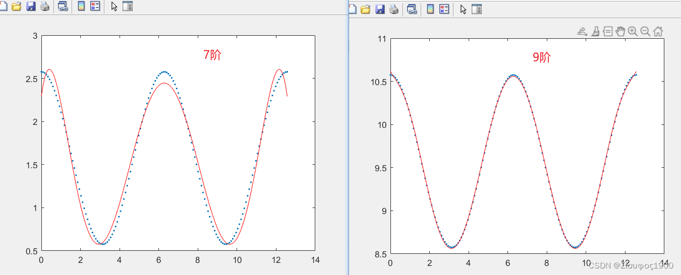
 从上图我们可以看出9阶的拟合效果要比7阶的好很多，那么我们用c++实现的时候也就按照9阶的来。