matlab图像处理

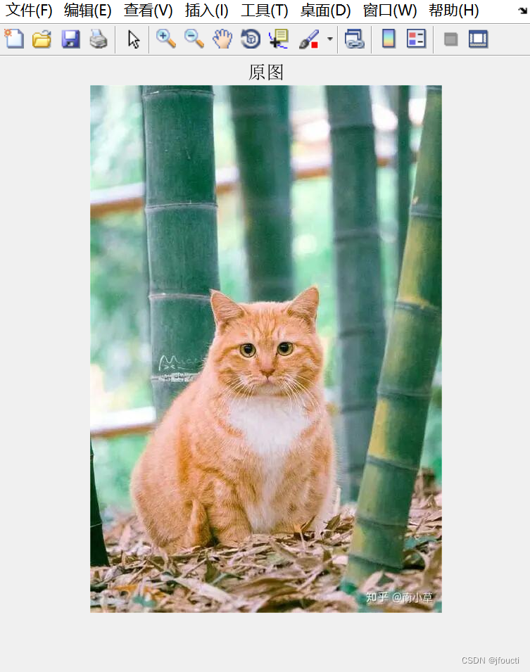
1.图片的读取（下左）

I=imread('可爱猫咪.jpg');%图像读取，这里''内为'路径\名称',如：'E:\examples\可爱猫咪.jpg'
figure,imshow(I);%图像显示
title('原图')

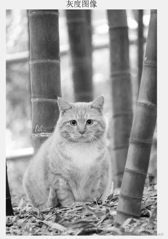
2.转为灰度图像（上右）

I_gray=rgb2gray(I);
figure,imshow(I_gray);
title('灰度图像')

查看是否是灰度图像的一个方法：

disp('输出字符串')%输出字符串；

ndims（）%输出矩阵维度，这里灰度图像或二值图像矩阵维度都为2，彩色图像为3。所以无法判断是灰度图像还是二值图像。之前matlab有函数isgray()，现在被移除了，就用如下办法将就吧。

imwrite(I,'I_gray.jpg')%将I保存为名为I_gray的.jpg图像.

if(ndims(I)==2)
    disp('是灰度图');
    imwrite(I,'I_gray.jpg')
else 
    disp('不是灰度图')
    Ig=rgb2gray(I);%转为灰度图Ig
    imwrite(Ig,'I_gray.jpg')
end

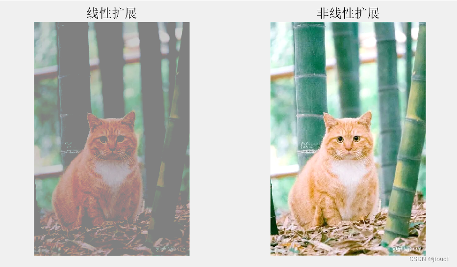
 3.线性扩展

a=0.6;
b=1;
c=0.5;
d=0.8; 
J=imadjust(I,[a;b],[c;d]);
subplot(1,2,1);%画布1行2列，放在第一个
imshow(J);
title('线性扩展');

4.非线性扩展

C=1.5;
K=C*log(1+((double(I))/255));%图像归一化处理
subplot(1,2,2);%画布1行2列，放在第二个
imshow(K);
title('非线性扩展');

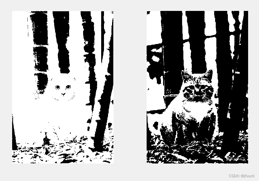
 5.二值化

N1=im2bw(I,0.4);
N2=im2bw(I,0.7);
subplot(1,2,1);
imshow(N1);
subplot(1,2,2);
imshow(N2);

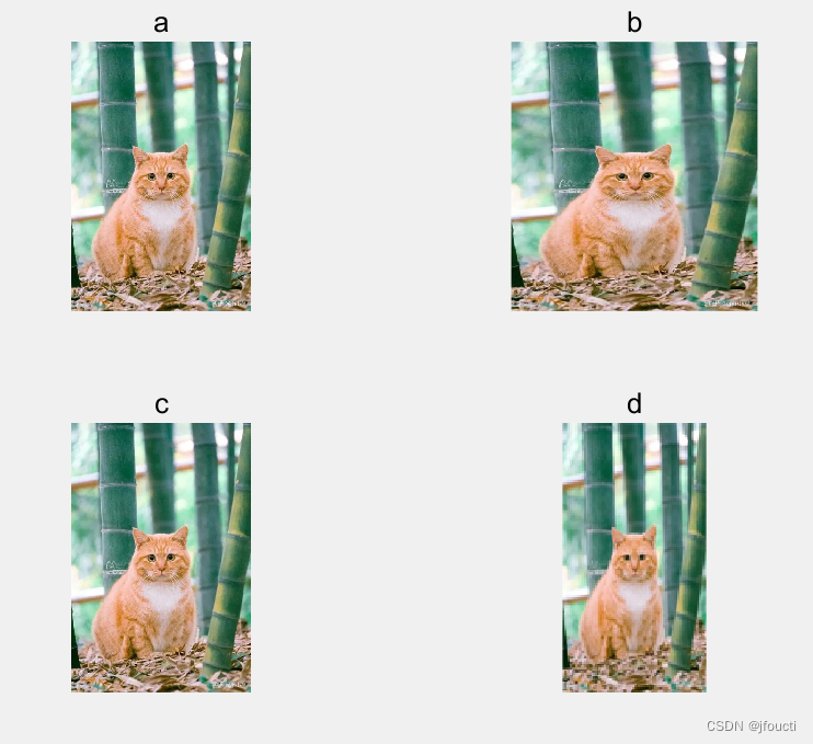
6.缩放

a=imresize(I,1.5);%按比例放大到1.5倍
b=imresize(I,[420,384]);%非比例
c=imresize(I,0.7);%按比例缩小到0.7倍
d=imresize(I,[150,80]);
subplot(2,2,1);
imshow(a);
title('a');
subplot(2,2,2);
imshow(b);
title('b');
subplot(2,2,3);
imshow(c);
title('c');
subplot(2,2,4);
imshow(d);
title('d');

 （噢，猫猫~）

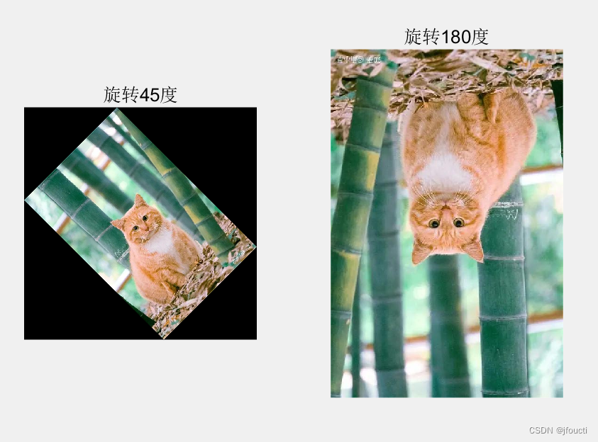
 7.旋转

K=imrotate(I,45);
subplot(1,2,1);
imshow(K);
title('旋转45度');
L=imrotate(I,180);
subplot(1,2,2);
imshow(L);
title('旋转180度');

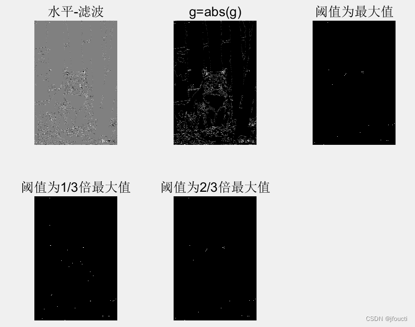
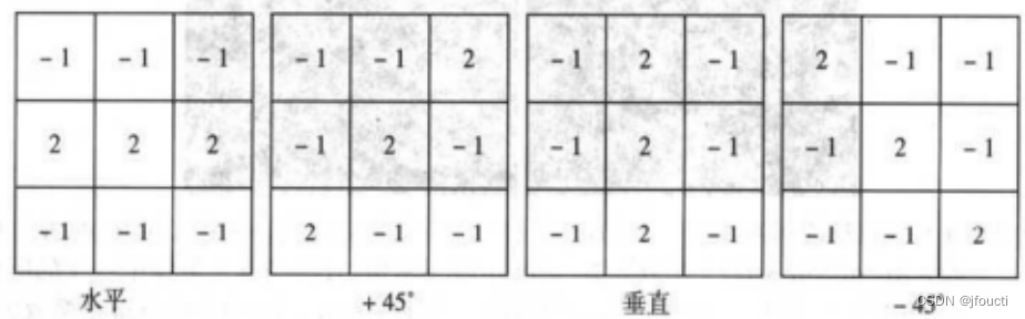
 8.线检测

此处代码为检测水平方向的线，可根据注释模板替换检测垂直等方向的线

I=im2bw(I,0.7);%此处应先将图像二值化或转为灰度图像
w=[-1 -1 -1; 2 2 2; -1 -1 -1];%水平
% w=[-1 -1 2; -1 2 -1; 2 -1 -1];%垂直
% w=[-1 2 -1; -1 2 -1; -1 2 -1];%45度
% w=[2 -1 -1; -1 2 -1; -1 -1 2];%-45度
g=imfilter(double(I), w);
figure,subplot(2,3,1);
imshow(g,{})  % 滤波后图像
title('水平-滤波')
g=abs(g);
subplot(2,3,2);
imshow(g,{})
title('g=abs(g)')
T=max(g(:));
g=g>=T;
subplot(2,3,3);
imshow(g)
title('阈值为T')
T=(1/3)*max(g(:));
g=g>=T;
subplot(2,3,4);
imshow(g)
title('阈值为1/3最大值')
T=(2/3)*max(g(:));
g=g>=T;
subplot(2,3,5);
imshow(g)
title('阈值为2/3最大值')

掩模例：

9.边缘检测

        edge()函数

        如：BW = edge(I,'prewitt',THRESH,DIRECTION) 表示对图像I，用prewitt方法；

        THRESH：规定了普鲁伊特prewitt方法的灵敏度阈值。边缘忽略所有不强于THRESH的边缘。如果你没有指定THRESH，或者THRESH为空， edge 会自动选择这个值。

         DIRECTION：寻找 "水平horizontal "或 "垂直 vertical"边缘，或 "两者"（默认）。

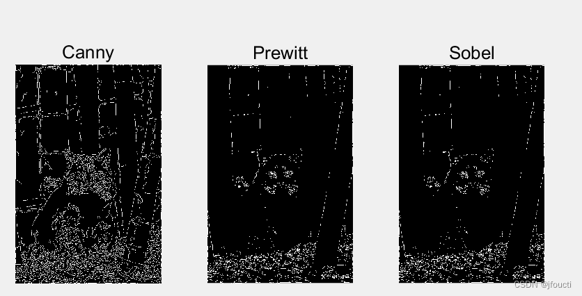
测试三种method，Canny,Prewitt,Sobel

I_gray=rgb2gray(I);%此处应先将图像二值化或转为灰度图像
a=edge(I_gray,'Canny');
b= edge(I_gray,'Prewitt');
c=edge(I_gray,'Sobel');
subplot(1,3,1);
imshow(a);
title('Canny');
subplot(1,3,2);
imshow(b);
title('Prewitt');
subplot(1,3,3);
imshow(c);
title('Sobel');

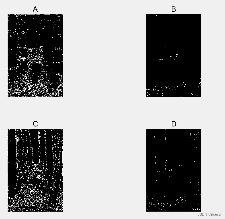
测试不同方向和不同阈值:

A=edge(I_gray,'Prewitt',0.02,'horizontal');
B=edge(I_gray,'Prewitt',0.15,'horizontal');
C=edge(I_gray,'Prewitt',0.02,'vertical');
D=edge(I_gray,'Prewitt',0.1,'vertical');
subplot(2,2,1);
imshow(A);
subplot(2,2,2);
imshow(B);
subplot(2,2,3);
imshow(C);
subplot(2,2,4);
imshow(D);

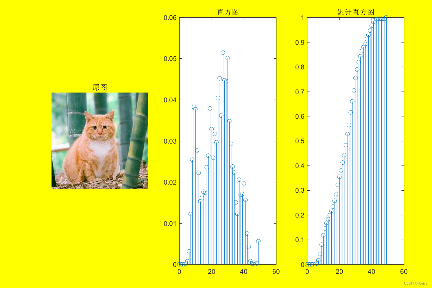
10.归一化直方图和累积直方图

I=imread('可爱猫咪.jpg');
set(gcf, 'Position', [20 70 900 600], 'color','y'); 
subplot(1,3,1),imshow(I),title('原图')
N=50;
Hist_image=imhist(img_gray,N); % 计算直方图
Hist_image=Hist_image/sum(Hist_image); % 计算归一化直方图
Hist_image_cumulation=cumsum(Hist_image); % 计算累计直方图
subplot(1,3,2),stem(0:N-1,Hist_image),title('直方图')
subplot(1,4,3),stem(0:N-1,Hist_image_cumulation),title('累计直方图')

这里为二次编辑，将图片裁剪为方形了。

set(gcf, 'Position', [20 70 900 600], 'color','y'); 

设置了figure位置：起始坐标为（20 ，70 ），宽度900，高度600像素。'color','y' 设置了图片背景为黄色 ，默认白色。（'r'是红色，'b'是蓝色，'w'白色）

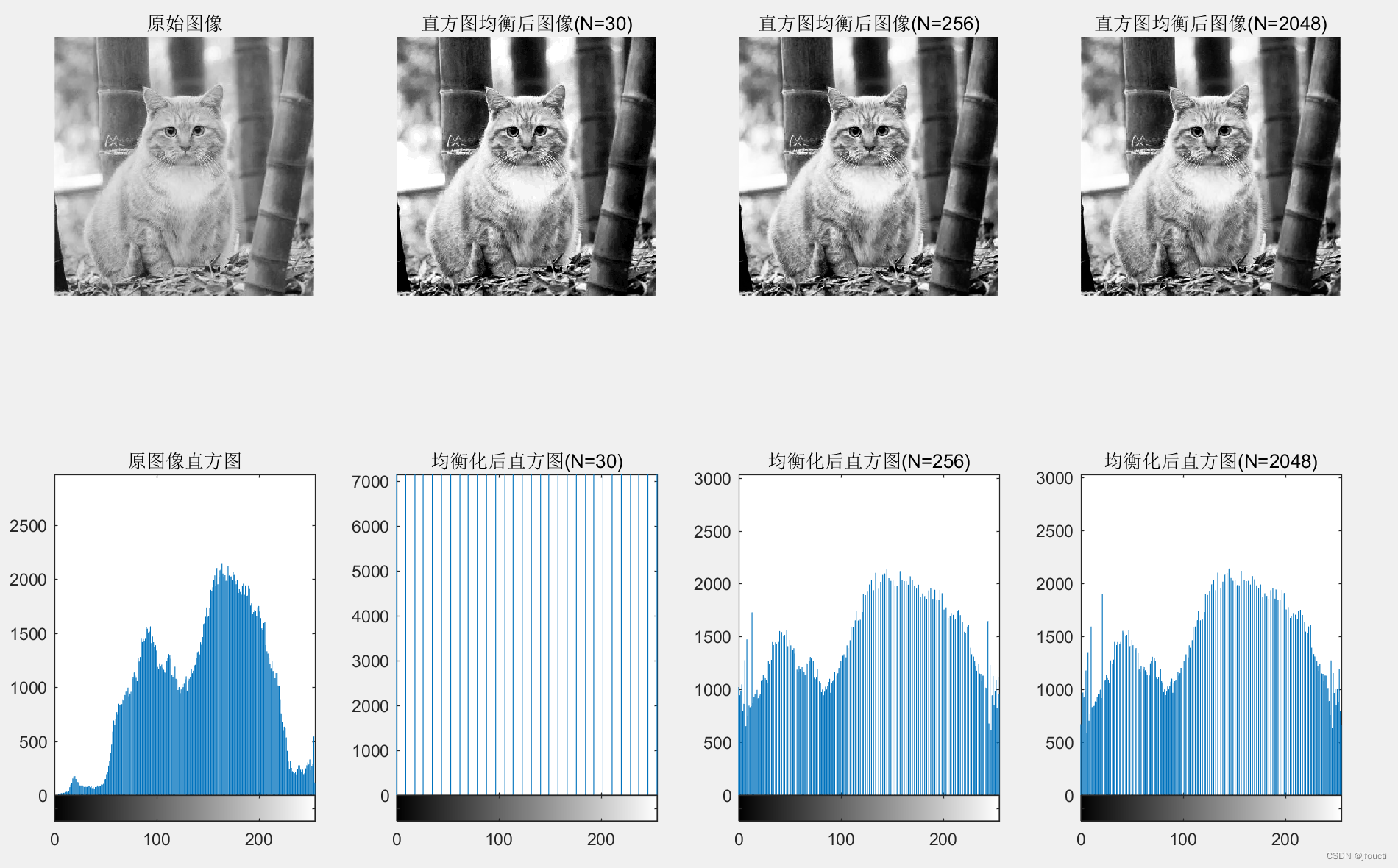
11. 直方图的均衡化

I=imread('可爱猫咪.jpg');
I_gray=rgb2gray(I);
subplot(2,4,1),imshow(I_gray),title('原始图像')
subplot(2,4,5),imhist(I_gray),title('原图像直方图')
N=30;
g=histeq(I_gray,N); % histeq 均衡化函数
subplot(2,4,2),imshow(g),title('直方图均衡后图像(N=30)')
subplot(2,4,6),imhist(g),title('均衡化后直方图(N=30)')
N=256;
g=histeq(I_gray,N); % histeq 均衡化函数
subplot(2,4,3),imshow(g),title('直方图均衡后图像(N=256)')
subplot(2,4,7),imhist(g),title('均衡化后直方图(N=256)')
N=2048;
g=histeq(I_gray,N); % histeq 均衡化函数
subplot(2,4,4),imshow(g),title('直方图均衡后图像(N=2048)')
subplot(2,4,8),imhist(g),title('均衡化后直方图(N=2048)')

12规定化直方图

I=imread('可爱猫咪.jpg');
I_gray=rgb2gray(I);
subplot(3,3,1),imshow(I_gray),title('原始图像')
subplot(3,3,7),imhist(I_gray),title('原图像直方图')
%幂函数变换直方图
Index=0:N-1;
Hist{1}=exp(-(Index-15).^2/8);  % 4
Hist{1}=Hist{1}/sum(Hist{1});
Hist_cumulation{1}=cumsum(Hist{1});
subplot(3,3,5),stem(0:N-1,Hist{1}),title('幂函数变换直方图')
% log函数直方图
Index=0:N-1;
Hist{2}=log(Index+20)/60;  % 15
Hist{2}=Hist{2}/sum(Hist{2});
Hist_cumulation{2}=cumsum(Hist{2});
subplot(3,3,6),stem(0:N-1,Hist{2}),title('log函数变换直方图')
 
% 规定化处理
for m=1:2
    Image=I_gray;
    for k=1:N
        Temp=abs(Hist_image_cumulation(k)-Hist_cumulation{m});
        [Temp1, Project{m}(k)]=min(Temp);
    end
    % 变换后直方图
    for k=1:N
        Temp=find(Project{m}==k); 
        if isempty(Temp)
            Hist_result{m}(k)=0;
        else
            Hist_result{m}(k)=sum(Hist_image(Temp));
        end
    end
    subplot(3,3,m+7),stem(0:N-1,Hist_result{m}),title('变换后直方图')
    % 结果图
    Step=256/N;
    for k=1:N
        Index=find(I_gray>=Step*(k-1)&I_gray