0. 前言
2022年没有新写什么博客, 主要精力都在搞论文. 今年开始恢复!
本文的目标是详细分析一个经典的基于landmark(文章后面有时也称之为控制点control point)的图像warping(扭曲/变形)算法: Thin Plate Spine (TPS).
TPS被广泛的应用于各类的任务中, 尤其是生物形态中应用的更多: 人脸, 动物脸等等, TPS是cubic spline的2D泛化形态. 值得注意的是, 图像处理中常用的仿射变换(Affine Transformation), 可以理解成TPS的一个特殊的变种.
- 什么是图像扭曲/变形问题?[3]
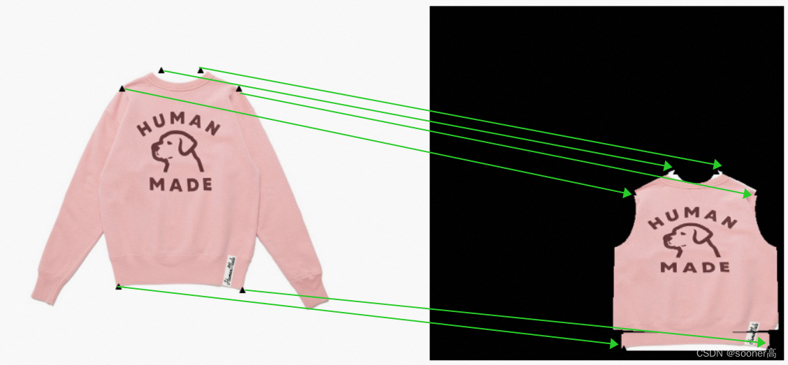
给定两张图片中一些相互对应的控制点(landmark, 如图绿色连接线所示),将 图片A(参考图像) 进行特定的形变,使得其控制点可以与 图片B(目标模板) 的landmark重合.
TPS是其中较为经典的方法, 其基础假设是:
如果用一个薄钢板的形变来模拟这种2D形变, 在确保landmarks能够尽可能匹配的情况下,怎么样才能使得钢板的弯曲量(deflection)最小。
- 用法示例
TPS算法在我的实践中, 用法是: 根据图像的landmark(下图左黑色三角), 将2D图像按照映射关系(绿色连接线)到的逻辑变形(warping)到目标模板(下图右).
1. 理论
Thin-Plate-Spline, 本文剩余部分均用其简称TPS来替代. TPS其实是一个数学概念[1]:
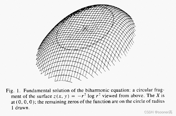
TPS是1D cubic spline的二维模拟, 它是 双调和方程 (Biharmonic Equation)[2]的基本解, 其形式如下:
U ( r ) = r 2 ln ( r ) U(r) = r^2 \ln(r) U(r)=r2ln(r)
1.1 U ( r ) U(r) U(r)形式的由来
那么为什么形式是这样的呢? Bookstein[10]在1989年发表的论文 “Principle Warps: Thin-Plate Splines and the Decomposition of Deformation” 中以双调和函数(Biharmonic Equation)的基础解进行展开:
首先, r r r表示的是 x 2 + y 2 \sqrt{x^2+y^2} x2+y2 (笛卡尔坐标系), 在论文中, Bookstein用的是 U ( r ) = − r 2 ln ( r ) U(r) = -r^2 \ln(r) U(r)=−r2ln(r), 其目的只是为了可视化方便: In this pose, it appears to be a slightly dented but otherwise convex surface viewed from above(即为了看起来中心X点附近的区域是一种 凹陷(dented) 的感觉).
这个函数天然的满足如下方程:
Δ 2 U = ( ∂ 2 ∂ x 2 + ∂ 2 ∂ y 2 ) 2 U ∝ δ ( 0 , 0 ) \Delta^2U = (\frac{\partial ^{2}}{\partial x^{2}} + \frac{\partial ^{2}}{\partial y^{2}})^2 U \propto \delta_{(0,0)} Δ2U=(∂x2∂2+∂y2∂2)2U∝δ(0,0)
公式的左侧和(0,0)的泛函 δ ( 0 , 0 ) \delta_{(0,0)} δ(0,0)等价(泛函介绍如下), δ ( 0 , 0 ) \delta_{(0,0)} δ(0,0)是在除了(0,0)处不等于0外, 任何其它位置都为0的泛函, 其积分为1(我猜, 狄拉克δ函数应该可以理解成这个泛函的一个形态).
所以, 由于双调和函数(Biharmonic Equation)的形式就是 Δ 2 U = 0 \Delta^2U=0 Δ2U=0, 那么显然, U ( r ) = ( ± ) r 2 ln ( r ) U(r) = (\pm) r^2 \ln(r) U(r)=(±)r2ln(r)都满足这个条件, 所以它被成为双调和函数的基础解(fundamental solution).
泛函简单来说, 就是定义域为函数集,而值域为实数或者复数的映射, 从知乎[11]处借鉴来一个泛函的例子:2D平面的两点之间直线距离最短.
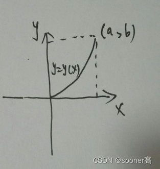
如图所示二维平面空间,从坐标原点(0,0)到点(a,b)的连接曲线是 y = y ( x ) y = y(x) y=y(x), 而连接曲线的微元 Δ \Delta Δ或者 d s = 1 + ( d y d x ) 2 d x ds = \sqrt{1+(\frac{dy}{dx})^2dx} ds=1+(dxdy)2dx , 对总的长度, 即为 d s ds ds在 [ 0 , a ] [0, a] [0,a]上的积分:
s = ∫ 0 a ( 1 + y ′ 2 ) 1 / 2 d x s = \int_{0}^{a}(1+y^{'2})^{1/2}dx s=∫0a(1+y′2)1/2dx 这里, s s s是标量(scalar), y ′ ( x ) y^{'}(x) y′(x)就是泛函(functional), 通常也记作 s ( y ′ ) s(y^{'}) s(y′). 那么上面的问题就转变成: 找出一条曲线 y ( x ) y(x) y(x),使得泛函 s ( y ′ ) s(y^{'}) s(y′)最小.
好的, U U U的来源和定义清楚了, 那么我们的目标是:
给定一组样本点,以每个样本点为中心的薄板样条(TPS)的加权组合给出了精确地通过这些点的插值函数,同时使所谓的弯曲能量(bending energy) 最小化.
那么, 什么是所谓的弯曲能量呢?
1.2 弯曲能量: Bending Energy
根据[1], 弯曲能量在这里定义为二阶导数的平方对实数域 R 2 R^2 R2(在我看来, 这里的 R 2 R^2 R2可以直接理解成2D image的Height and Width, 即高度和宽度)的积分:
I [ f ( x , y ) ] = ∬ ( f x x 2 + 2 f x y 2 + f y y 2 ) d x d y I[f(x, y)] = \iint (f_{xx}^2 + 2f_{xy}^2+ f_{yy}^2)dxdy I[f(x,y)]=∬(fxx2+2fxy2+fyy2)dxdy
优化的目标是要让 I [ f ( x , y ) ] I[f(x, y)] I[f(x,y)]最小化.
好了, 弯曲能量的数学定义到此结束, 很自然的,我们会如下的疑问:
- f ( x , y ) f(x, y) f(x,y)是如何定义的?
- 对图像这样的2D平面, 其样条的加权组合后的弯曲的方向应该是什么样的, 才能使得弯曲能量最小?
首先我们先分析下弯曲的方向的问题, 并在1.4中进行 f ( x , y ) f(x, y) f(x,y)定义的介绍.
1.3 弯曲的方向
首先, 回顾一下TPS的命名, TPS起源于一个物理的类比: the bending of a thin sheet of metal (薄金属片的弯曲).
在物理学上来讲, 弯曲的方向(deflection)是 z z z轴, 即垂直于2D图像平面的轴.
为了将这个idea应用于坐标转换的实际问题当中, 我们将TPS理解成是将平板进行拉升 or 降低, 再将拉升/降低后的平面投影到2D图像平面, 即得到根据参考图像和目标模板的landmark对应关系进行warping(形变)后的图像结果.
如下所示, 将平面上设置4个控制点, 其中最后一个不是边缘角点, 在做拉扯的时候, 平面就自然产生了一种局部被拉高或者降低的效果.
显然, 这种warping在一定程度上也是一种坐标转换(coordinate transformation), 如下图所示, 给定参考landmark红色 X X X和目标点蓝色 ⚪ ⚪ ⚪. TPS warping将会将这些 X X X完美的移动到 ⚪ ⚪ ⚪上.
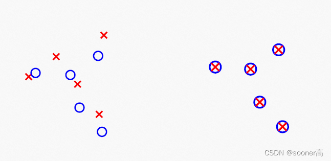
问题来了, 那么这个 X → ⚪ X \rightarrow ⚪ X→⚪移动的方案是如何实现的呢?
1.4 如何实现2D plane的coordinate transformation (a.k.a warping)?
如下图[7], 2D plane上的坐标变换其实就是2个方向的变化: X \mathbf{X} X 和 Y \mathbf{Y} Y方向. 来实现这2个方向的变化, TPS的做法是:
用2个样条函数分别考虑 X \mathbf{X} X和 Y \mathbf{Y} Y方向上的位移(displacement).
TPS actually use two splines,
one for the displacement in the X direction
and one for the displacement in the Y direction
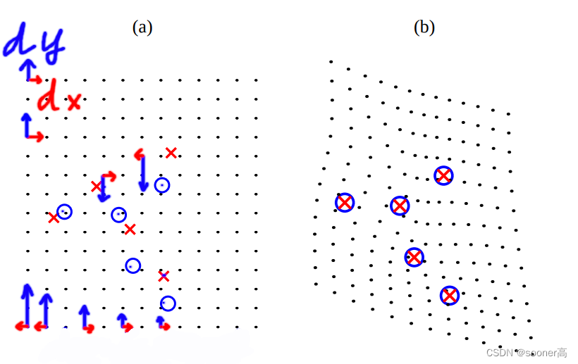
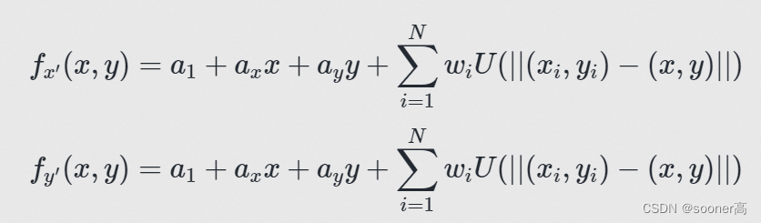
这2个样条函数的定义如下[7] ( N N N指的是对应的landmark数量, 如上图所示, N = 5 N=5 N=5):
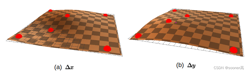
注意, 每个方向( X , Y \mathbf{X}, \mathbf{Y} X,Y)的位移( Δ X , Δ Y \mathbf{\Delta X}, \mathbf{\Delta Y} ΔX,ΔY)可以被视为 N N N个点高度图(height map), 因此样条的就像在3D空间拟合 散点(scatter point) 一样, 如下图所示[7].
在样条函数的定义公式中,
- 前3个系数 a 1 , a x , a y a_1, a_x, a_y a1,ax,ay表示线性空间的部分(line part), 用于在线性空间拟合 X X X ( x i , y i x_i, y_i xi,yi)和 ⚪ ⚪ ⚪ ( x i ′ , y i ′ x_i^{'}, y_i^{'} xi′,yi′).
- 紧接着的系数 w i , i ∈ [ 1 , N ] w_i, i \in [1, N] wi,i∈[1,N]表示每个控制点 i i i的kernel weight, 它用于乘以控制点 X X X ( x i , y i x_i, y_i xi,yi)和其最终的 x , y x, y x,y之间的位移(displacement).
- 最后的一项是
U
(
∣
∣
(
x
i
,
y
i
)
−
(
x
,
y
)
∣
∣
)
U(|| (x_i, y_i) - (x, y) ||)
U(∣∣(xi,yi)−(x,y)∣∣), 即控制点
X
X
X (
x
i
,
y
i
x_i, y_i
xi,yi)和其最终的
x
,
y
x, y
x,y之间的位移. 需要注意的是,
U
(
∣
∣
(
x
i
,
y
i
)
−
(
x
,
y
)
∣
∣
)
U(|| (x_i, y_i) - (x, y) ||)
U(∣∣(xi,yi)−(x,y)∣∣)用的是L2范数[8]. 这里
U
U
U定义如下:
U
(
r
)
=
r
2
ln
(
r
)
U(r) = r^2 \ln(r)
U(r)=r2ln(r) 这里我们需要revisit一下TPS的RBF函数(radial basis function) :
U
(
r
)
=
r
2
ln
(
r
)
U(r) = r^2 \ln(r)
U(r)=r2ln(r) , 根据[9]所述, 像RBF这种Gaussian Kernel, 是一种用于衡量相似性的方法(Similarity measurement).
1.5 具体计算方案
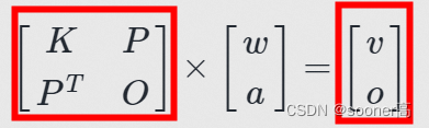
对于每个方向( X , Y \mathbf{X}, \mathbf{Y} X,Y)的样条函数的系数 a 1 , a x , a y , w i a_1, a_x, a_y, w_i a1,ax,ay,wi, 可以通过求解如下linear system来获得:
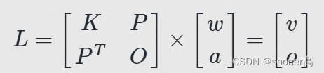
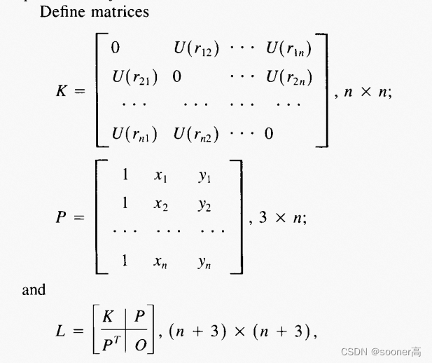
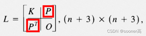
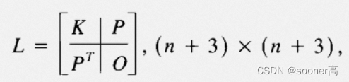
其中, K i j = U ( ∣ ∣ ( x i , y i ) − ( x j , y j ) ∣ ∣ ) K_{ij} = U(|| (x_i, y_i) - (x_j, y_j) ||) Kij=U(∣∣(xi,yi)−(xj,yj)∣∣), P P P的第 i i i行是齐次表示 ( 1 , x i , y i ) (1, x_i, y_i) (1,xi,yi), O O O是3x3的全0矩阵, o o o是3x1的全0列向量, w w w和 v v v是 w i w_i wi和 v i v_i vi组成的列向量. a a a是由 [ a 1 , a x , a y ] [a_1, a_x, a_y] [a1,ax,ay]组成的列向量.
具体地, 左侧的大矩阵形式如下[9-10]:
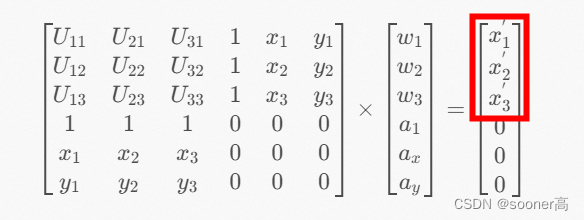
以N=3(控制点数量为3)为例, X \mathbf{X} X方向的样条函数的线性矩阵表达为:
[ U 11 U 21 U 31 1 x 1 y 1 U 12 U 22 U 32 1 x 2 y 2 U 13 U 23 U 33 1 x 3 y 3 1 1 1 0 0 0 x 1 x 2 x 3 0 0 0 y 1 y 2 y 3 0 0 0 ] × [ w 1 w 2 w 3 a 1 a x a y ] = [ x 1 ′ x 2 ′ x 3 ′ 0 0 0 ] \begin{bmatrix} U_{11} & U_{21} & U_{31} & 1 & x_1 & y_1\\ U_{12} & U_{22} & U_{32} & 1 & x_2 & y_2\\ U_{13} & U_{23} & U_{33} & 1 & x_3 & y_3 \\ 1 & 1 & 1 & 0 & 0& 0 \\ x_1 & x_2 & x_3 & 0 & 0& 0 \\ y_1 & y_2 & y_3 & 0 & 0& 0 \end{bmatrix} \times \begin{bmatrix} w_1 \\ w_2 \\ w_3 \\ a_1 \\ a_x \\ a_y \end{bmatrix} = \begin{bmatrix} x_1^{'} \\ x_2^{'} \\ x_3^{'} \\ 0 \\ 0 \\ 0 \end{bmatrix} U11U12U131x1y1U21U22U231x2y2U31U32U331x3y3111000x1x2x3000y1y2y3000 × w1w2w3a1axay = x1′x2′x3′000
同样地, Y \mathbf{Y} Y的样条函数的线性矩阵表达为:
[ U 11 U 21 U 31 1 x 1 y 1 U 12 U 22 U 32 1 x 2 y 2 U 13 U 23 U 33 1 x 3 y 3 1 1 1 0 0 0 x 1 x 2 x 3 0 0 0 y 1 y 2 y 3 0 0 0 ] × [ w 1 w 2 w 3 a 1 a x a y ] = [ y 1 ′ y 2 ′ y 3 ′ 0 0 0 ] \begin{bmatrix} U_{11} & U_{21} & U_{31} & 1 & x_1 & y_1\\ U_{12} & U_{22} & U_{32} & 1 & x_2 & y_2\\ U_{13} & U_{23} & U_{33} & 1 & x_3 & y_3 \\ 1 & 1 & 1 & 0 & 0& 0 \\ x_1 & x_2 & x_3 & 0 & 0& 0 \\ y_1 & y_2 & y_3 & 0 & 0& 0 \end{bmatrix} \times \begin{bmatrix} w_1 \\ w_2 \\ w_3 \\ a_1 \\ a_x \\ a_y \end{bmatrix} = \begin{bmatrix} y_1^{'} \\ y_2^{'} \\ y_3^{'} \\ 0 \\ 0 \\ 0 \end{bmatrix} U11U12U131x1y1U21U22U231x2y2U31U32U331x3y3111000x1x2x3000y1y2y3000 × w1w2w3a1axay = y1′y2′y3′000
显然可见, N+3个函数来求解N+3个未知量, 能得到相应的 [ w a ] \begin{bmatrix} w \\ a \end{bmatrix} [wa].
2. 代码实现
我使用的TPS是cheind/py-thin-plate-spline项目[6], 这里会对代码进行详细拆解, 以达到理解公式和实现的对应关系.
2.1 核心计算逻辑
核心逻辑在函数warp_image_cv中: tps.tps_theta_from_points, tps.tps_grid和tps.tps_grid_to_remap,
最基本的示例代码如下:
def show_warped(img, warped, c_src, c_dst):
    fig, axs = plt.subplots(1, 2, figsize=(16,8))
    axs[0].axis('off')
    axs[1].axis('off')
    axs[0].imshow(img[...,::-1], origin='upper')
    axs[0].scatter(c_src[:, 0]*img.shape[1], c_src[:, 1]*img.shape[0], marker='^', color='black')
    axs[1].imshow(warped[...,::-1], origin='upper')
    axs[1].scatter(c_dst[:, 0]*warped.shape[1], c_dst[:, 1]*warped.shape[0], marker='^', color='black')
    plt.show()
def warp_image_cv(img, c_src, c_dst, dshape=None):
    dshape = dshape or img.shape
    theta = tps.tps_theta_from_points(c_src, c_dst, reduced=True)
    grid = tps.tps_grid(theta, c_dst, dshape)
    mapx, mapy = tps.tps_grid_to_remap(grid, img.shape)
    return cv2.remap(img, mapx, mapy, cv2.INTER_CUBIC)
img = cv2.imread('test.jpg')
c_src = np.array([
    [0.44, 0.18],
    [0.55, 0.18],
    [0.33, 0.23],
    [0.66, 0.23],
    [0.32, 0.79],
    [0.67, 0.80],
])
c_dst = np.array([
    [0.693, 0.466],
    [0.808, 0.466],
    [0.572, 0.524],
    [0.923, 0.524],
    [0.545, 0.965],
    [0.954, 0.966],
])
warped_front = warp_image_cv(img, c_src, c_dst, dshape=(512, 512))
show_warped(img, warped1, c_src_front, c_dst_front)
此开源代码有2个版本: numpy和torch. 这里我的分析以numpy版本进行, 以便没有GPU用的朋友进行hands-on的测试.
核心类TPS
class TPS:
  @staticmethod
   def fit(c, lambd=0., reduced=False):
      n = c.shape[0]
      U = TPS.u(TPS.d(c, c))
      K = U + np.eye(n, dtype=np.float32)*lambd
      P = np.ones((n, 3), dtype=np.float32)
      P[:, 1:] = c[:, :2]
      v = np.zeros(n+3, dtype=np.float32)
      v[:n] = c[:, -1]
       A = np.zeros((n+3, n+3), dtype=np.float32)
       A[:n, :n] = K
       A[:n, -3:] = P
       A[-3:, :n] = P.T
       theta = np.linalg.solve(A, v) # p has structure w,a
       return theta[1:] if reduced else thete
       ...
   @staticmethod
   def z(x, c, theta):
       x = np.atleast_2d(x)
       U = TPS.u(TPS.d(x, c))
       w, a = theta[:-3], theta[-3:]
       reduced = theta.shape[0] == c.shape[0] + 2
       if reduced:
           w = np.concatenate((-np.sum(w, keepdims=True), w))
       b = np.dot(U, w)
       return a[0] + a[1]*x[:, 0] + a[2]*x[:, 1] + b
2.2 tps.tps_theta_from_points
此函数的作用是为了求解样条函数的 [ w a ] \begin{bmatrix} w \\ a \end{bmatrix} [wa].
def tps_theta_from_points(c_src, c_dst, reduced=False): delta = c_src - c_dst cx = np.column_stack((c_dst, delta[:, 0])) cy = np.column_stack((c_dst, delta[:, 1])) theta_dx = TPS.fit(cx, reduced=reduced) theta_dy = TPS.fit(cy, reduced=reduced) return np.stack((theta_dx, theta_dy), -1)-
delta 是 在参考图的控制点和目标模板的控制点之间的插值 Δ x i , Δ y i \Delta x_i, \Delta y_i Δxi,Δyi
-
cx和cy是在c_dst的基础上, 分别加了 Δ x i \Delta x_i Δxi和 Δ y i \Delta y_i Δyi的列向量
-
theta_dx和theta_dy的reduce参数默认为False/True时. 其结果是1D向量, 长度为9/8 . 其计算过程需要看TPS核心类的fit函数.
① TPS.d(cx, cx, reduced=True) or TPS.d(cy, cy, reduced=True) 计算L2
    @staticmethod
    def d(a, b):
        # a[:, None, :2] 是把a变成[N, 1, 2]的tensor/ndarray
        # a[None, :, :2] 是把a变成[1, N, 2]的tensor/ndarray
        return np.sqrt(np.square(a[:, None, :2] - b[None, :, :2]).sum(-1))
其作用是计算样条中的 ∣ ∣ ( x i , y i ) − ( x , y ) ∣ ∣ || (x_i, y_i) - (x, y) || ∣∣(xi,yi)−(x,y)∣∣ (L2), 得出的结果是shape为 N , N N, N N,N的中间结果.
② TPS.u(...) 计算 U ( . . . ) U(...) U(...)
和公式完全一样: U ( r ) = r 2 ln ( r ) U(r) = r^2 \ln(r) U(r)=r2ln(r), 为了防止 r r r太小, 加了个epsilon系数 1 e − 6 1e^{-6} 1e−6. 这一步得到 K K K, shape仍然是 N , N N, N N,N, 和①一样.
def u(r):
        return r**2 * np.log(r + 1e-6)
③ 根据cx和cy, 简单拼接即可生成P.
	P = np.ones((n, 3), dtype=np.float32)
	P[:, 1:] = c[:, :2] # c就是cx or cy.
④ 根据 Δ x i \Delta x_i Δxi (cx得最后一列向量, cy同理), 得到 v v v
    # c = cx or cy
    v = np.zeros(n+3, dtype=np.float32)
    v[:n] = c[:, -1]
⑤ 组装矩阵A, 即[10]论文中的 L L L矩阵.
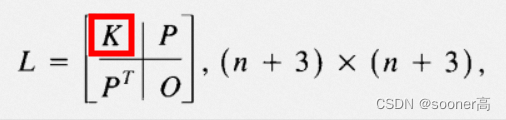
     A = np.zeros((n+3, n+3), dtype=np.float32)
     A[:n, :n] = K
     A[:n, -3:] = P
     A[-3:, :n] = P.T
⑥ 现在 L L L和 Y Y Y已知, Y = [ v o ] Y = \begin{bmatrix}v \\ o \end{bmatrix} Y=[vo], 那么 W W W和 a 1 , a x , a y a_1, a_x, a_y a1,ax,ay的向量可以直接线性求解
[ w a ] \begin{bmatrix}w \\ a \end{bmatrix} [wa] = L − 1 L^{-1} L−1 Y Y Y
class TPS:
    @staticmethod
    def fit(c, lambd=0., reduced=False):
        # 1. TPS.d
        U = TPS.u(TPS.d(c, c))
        K = U + np.eye(n, dtype=np.float32)*lambd
        P = np.ones((n, 3), dtype=np.float32)
        P[:, 1:] = c[:, :2]
        v = np.zeros(n+3, dtype=np.float32)
        v[:n] = c[:, -1]
        A = np.zeros((n+3, n+3), dtype=np.float32)
        A[:n, :n] = K
        A[:n, -3:] = P
        A[-3:, :n] = P.T
        theta = np.linalg.solve(A, v) # p has structure w,a
        return theta[1:] if reduced else theta

    @staticmethod
    def d(a, b):
        return np.sqrt(np.square(a[:, None, :2] - b[None, :, :2]).sum(-1))
    @staticmethod
    def u(r):
        return r**2 * np.log(r + 1e-6)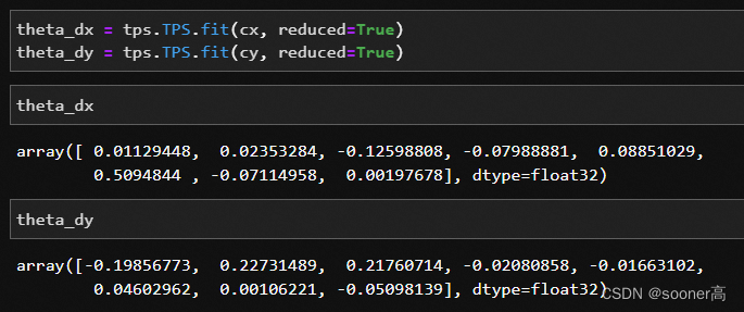
即函数返回的theta就是 [ w a ] \begin{bmatrix}w \\ a \end{bmatrix} [wa]. 由于我们是2个方向(X, Y)都要这个theta, 因此
theta = tps.tps_theta_from_points(c_src, c_dst)
返回的theta是 ( N + 3 , 2 ) (N+3, 2) (N+3,2)的形式.
2.3 tps.tps_grid
此函数是为了求解image plane在x和y方向上的偏移量(offset).
def warp_image_cv(img, c_src, c_dst, dshape=None):
    dshape = dshape or img.shape
    # 2.2
    theta = tps.tps_theta_from_points(c_src, c_dst, reduced=True)
    # 2.3
    grid = tps.tps_grid(theta, c_dst, dshape)
    # 2.4
    mapx, mapy = tps.tps_grid_to_remap(grid, img.shape)
    return cv2.remap(img, mapx, mapy, cv2.INTER_CUBIC)
由核心代码部分可以看出, 当求出theta, 也就是 [ w a ] \begin{bmatrix}w \\ a \end{bmatrix} [wa]. 我们下面用tps_grid函数进行网格的warping操作.
函数如下:
def tps_grid(theta, c_dst, dshape):
    # 1) uniform_grid(...)
    ugrid = uniform_grid(dshape)
    reduced = c_dst.shape[0] + 2 == theta.shape[0]
    # 2) 求dx和dy.
    dx = TPS.z(ugrid.reshape((-1, 2)), c_dst, theta[:, 0]).reshape(dshape[:2])
    dy = TPS.z(ugrid.reshape((-1, 2)), c_dst, theta[:, 1]).reshape(dshape[:2])
    dgrid = np.stack((dx, dy), -1)
    grid = dgrid + ugrid

    return grid # H'xW'x2 grid[i,j] in range [0..1]
其输入是3个参数:
- theta reduced=True(N+2, 2) or reduced=False (N+3, 2)
- c_dst (N, 2), 是目标模板上的control points or landmarks.
c_dst = np.array([ [0.693, 0.466], [0.808, 0.466], [0.572, 0.524], [0.923, 0.524], [0.545, 0.965], [0.954, 0.966], ])- dshape (H, W, 3), 是给定参考图像的分辨率.
输出是1个:
- grid (H, W, 2).
其可视化效果见2.3.1.
2.3.1 uniform_grid
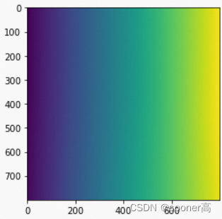
tps.tps_grid函数的第一步是ugrid = uniform_grid(dshape), 此函数的定义如下, 作用是创建1个 ( H , W , 2 ) (H, W, 2) (H,W,2)的grid, 里面的值都是0到1的线性插值np.linspace(0, 1, W(H)).
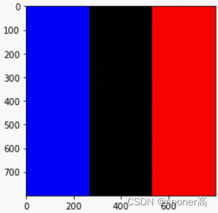
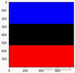
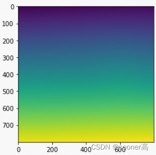
def uniform_grid(shape):
    '''Uniform grid coordinates.
    '''
    H,W = shape[:2]
    c = np.empty((H, W, 2))
    c[..., 0] = np.linspace(0, 1, W, dtype=np.float32)
    c[..., 1] = np.expand_dims(np.linspace(0, 1, H, dtype=np.float32), -1)
    return c
返回的ugrid就是一个 ( H , W , 2 ) (H, W, 2) (H,W,2)的grid, 其X, Y方向值的大小按方向线性展开, 如下图所示.
X方向
Y方向
2.3.2 TPS.z求解得到dx和dy
 # 2) 求dx和dy.
 dx = TPS.z(ugrid.reshape((-1, 2)), c_dst, theta[:, 0]).reshape(dshape[:2]) # [H, W]
 dy = TPS.z(ugrid.reshape((-1, 2)), c_dst, theta[:, 1]).reshape(dshape[:2]) # [H, W]
 dgrid = np.stack((dx, dy), -1)  # [H, W, 2]
 grid = dgrid + ugrid
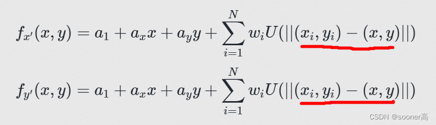
由下面的TPS.z定义容易看出, 这个函数就是求解X和Y方向的样条函数:
f ( x / y ) ′ ( x , y ) = a 1 + a x x + a y y + ∑ i = 1 N w i U ( ∣ ∣ ( x i , y i ) − ( x , y ) ∣ ∣ ) f_{(x/y)^{'}}(x, y) = a_1 + a_x x + a_y y + \sum_{i=1}^{N} w_i U(|| (x_i, y_i) - (x, y) ||) f(x/y)′(x,y)=a1+axx+ayy+i=1∑NwiU(∣∣(xi,yi)−(x,y)∣∣)
可能让人有困惑的点是说, 为什么在2.2的时候, TPS.d()的传参是一样的(cx(cy)), 而这里的x是shape为(H*W), 2, 而c仍旧是c_dst (N,2), 我的理解是说, 由于2.3这一步的目标是为了真正的让image plane按照控制点的位置进行移动(最小化弯曲能量), 所以通过ugrid均匀对平面采样的点进行offset计算(dx和dy), 使其得到满足推导条件下的offset解析解dgrid.
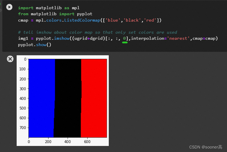
class TPS:
    ...
    @staticmethod
    def z(x, c, theta):
        x = np.atleast_2d(x)
        U = TPS.u(TPS.d(x, c)) # [H*W, N] 本例中H=W=800, N=6
        w, a = theta[:-3], theta[-3:]
        reduced = theta.shape[0] == c.shape[0] + 2
        if reduced:
            w = np.concatenate((-np.sum(w, keepdims=True), w))
        b = np.dot(U, w)
        return a[0] + a[1]*x[:, 0] + a[2]*x[:, 1] + b
所以对ugrid+dgrid, 即得到整个图像平面按照样条函数计算出来的 d x , d y dx, dy dx,dy(offset)加到均匀的ugrid的结果: 显然可以看出, 这个结果相比2.3.1的ugrid, 在 X , Y \mathbf{X}, \mathbf{Y} X,Y方向有了相应的变化.
X方向
Y方向
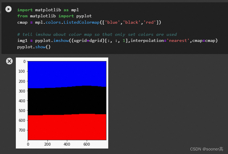
到这里, 2.3这步返回的其实就是一个在 X , Y \mathbf{X}, \mathbf{Y} X,Y方向相应扭曲的grid(格子) ( H , W , 2 ) (H, W, 2) (H,W,2), 其可视化结果如上, 值的范围都在 -1到1 之间.
2.4 tps.tps_grid_to_remap
这一步很简单了, 就是把2.3计算得到的**grid(格子)**按 X , Y \mathbf{X}, \mathbf{Y} X,Y方向分别乘以对应的 W W W和 H H H. 然后送去cv2.remap函数进行图像的扭曲操作.
def warp_image_cv(img, c_src, c_dst, dshape=None):
    dshape = dshape or img.shape
    # 2.2
    theta = tps.tps_theta_from_points(c_src, c_dst, reduced=True)
    # 2.3
    grid = tps.tps_grid(theta, c_dst, dshape)
    # 2.4
    mapx, mapy = tps.tps_grid_to_remap(grid, img.shape)
    return cv2.remap(img, mapx, mapy, cv2.INTER_CUBIC)
2.4.1 tps_grid_to_remap 简单的把grid乘以宽和高
def tps_grid_to_remap(grid, sshape):
    '''Convert a dense grid to OpenCV's remap compatible maps.
    Returns
    -------
    mapx : HxW array
    mapy : HxW array
    '''
    mx = (grid[:, :, 0] * sshape[1]).astype(np.float32)
    my = (grid[:, :, 1] * sshape[0]).astype(np.float32)
    return mx, my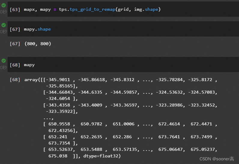
2.4.2 cv2.remap(img, mapx, mapy, cv2.INTER_CUBIC) 得到warp后的结果.
cv2.remap是允许用户自己定义映射关系的函数, 不同于通过变换矩阵进行的仿射变换和透视变换, 更加的灵活, TPS就是使用的这种映射. 具体示例参考[12].

需要注意的是, 这个结果之所以和前言中的不一样, 是因为在前言里, 我们用了mask来做遮罩.
总结
到这里, TPS的分析就告一段落了, 这种算法是瘦脸, 纹理映射等任务中最常见的, 也是很灵活的warping算法, 目前还仍然在广泛使用, 如果文章哪里写的有谬误或者问题, 欢迎大家在下面指出,
感谢 ^ . ^
参考文献
- Thin Plate Spline: MathWorld
- Biharmonic Equation: MathWorld
- c0ldHEart: Thin Plate Spline TPS薄板样条变换基础理解
- MIT: WarpMorph
- Approximation Methods for Thin Plate Spline Mappings and Principal Warps
- cheind/py-thin-plate-spline
- Thin-Plate-Splines-Warping
- Wikipedia: Thin plate spline
- Deep Shallownet: Radial Basis Function Kernel - Gaussian Kernel
- Bookstein: Principle Warps: Thin Plate Splines and the Decomposition of Deformations
- 知乎:「泛函」究竟是什么意思?
- 【opencv】5.5 几何变换-- 重映射 cv2.remap()
- grid (H, W, 2).
- dshape (H, W, 3), 是给定参考图像的分辨率.
-
- 用法示例